Fluid Mathematics

Man lives on land in a planet with a life-supporting atmosphere and many rivers and oceans. And we wonder at the mind-boggling diversity of the way in which air and water flow: clouds, tornadoes, dust devils, waterfalls, river bores, placid lakes, ocean waves, tsunamis, whirlpools… sometimes soothing, sometimes beautiful, sometimes fearsome, often turbulent. And the equations governing these fluid flows have been known for nearly two centuries. But today we still do not understand, and cannot satisfactorily predict, any turbulent flow—from the pressure drop in the pipe circulating water in our kitchen (the answer is known by experience, not by reasoning) to that wonderful, majestic cumulus cloud that can be called the queen of the tropical sky (after Riehl). As Feynman said, turbulence is the last great unsolved problem of classical physics. If the equations are known but the solutions are not, it is clearly a problem in mathematics—one case where mathematics has been singularly ineffective till now. So it is not such a great surprise perhaps that the Clay Foundation in the US has offered a prize of a million dollars for finding the answers to a fundamental mathematical problem in fluid mechanics. (By the way, how is it that we talk of fluid mechanics, fluid dynamics, fluid physics and fluids engineering but never of fluid mathematics, when the subject is really closely tied to mathematics, as I have just pointed out?)

The Prize is about limiting solutions of the Navier–Stokes equations (Box 1), which govern the flow of common fluids like air and water: mundane, classical, perhaps prosaic, you may think. Not so—as I hope to show you: for behind the mundane in this case lurks the arcane, in Michael Berry’s phrase about a certain kind of science.

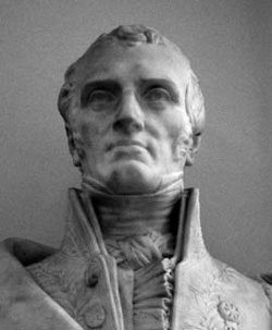
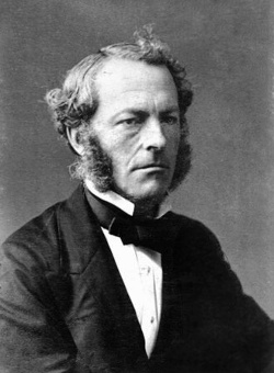
The equations were first written down by the French engineer Louis Navier in 1822, with a molecular argument that led to a momentum diffusion term. According to Navier this had nothing to do with viscosity. But in 1845 George Stokes derived the same partial differential equations as Navier did but appealing explicitly to viscosity, and to linear relations between stress and strain rate in an isotropic medium—very much as we would do it today. Between Navier and Stokes there were others who contributed; at any rate the equations had a fairly long gestation period of 23 years before acceptance (Figure 1). Finding the right boundary conditions took a little longer.

A solution to the Clay mathematical problem is actually going to help in engineering at some stage or the other. The reason is that the limit \nu \rightarrow 0 (vanishing viscosity) is very important for engineers. To see this, we must first realize that the relevant value of \nu is not what you get for any fluid in the hand books of physics: it is the value relevant to the flow problem, i.e., it should be expressed in the natural flow units velocity (U, say) \times length (L, say), not in meters and seconds. That is, as the British engineer Osborne Reynolds figured out in 1883, we really want the handbook value divided by UL, which gives us the reciprocal of what came to be called the Reynolds number. Using a flow-scaled \nu, a mainline Boeing aircraft would fly around \nu \sim 10^{-7}, birds at about 10^{-4}, the smallest insects at around 1. It is legitimate to ask: Is 10^{-7}, or 10^{-4} (or even 1) close to zero? (Equivalently, is the reciprocal, the Reynolds number, close to the limit of infinity at 10^{7}?)

But the answer is not obvious. To see this, look at how crazy and long the crooked road to \nu = 0 is for one particular fluid-dynamical parameter, namely the base pressure (more precisely, the nondimensionalized pressure coefficient at the rear stagnation point) on a perfect, smooth circular cylinder in a stream of given velocity (Figure 2). Who would have thought that the path from 10^{-1} to 10^{-7} (meticulously surveyed by Anatol Roshko in 1993) could be so full of ups and downs, zigs and zags?

Why is this so? The chief reason is: Because the non-linearity in the Navier–Stokes equations becomes more important as \nu \rightarrow 0 (the other limit \nu \rightarrow \infty is linear and boring (I am exaggerating)), and because the road is strewn with rocks known as regime transitions, some of them big boulders causing huge changes, and some little pebbles causing tiny kinks. Almost all of the nine transitions shown in the figure (labelled A to J) come from experimental data (acquired in several different labs across the world). Apart from the relatively smooth curve at the boring end of \nu there are no theories, and only one or two transitions at the same end of \nu can be computed at present. Here, incidentally, is the challenge to Fluid Mathematics and to computer science.

The most famous transition is from laminar to turbulent flow. This, by the way, was the main subject of that 1883 paper by Reynolds: transition to turbulence in pipe flow. (His paper on the subject began by pointing out that the problem was of both practical and philosophical interest; we could say the same thing today, more than a century later.) He showed that transition—and, as it turned out, the whole character of any flow—depended only on the Reynolds number combination, not on the fluid itself; thus a dust particle in air may behave like a marble in honey, for the Reynolds number can be the same in both cases, although (or because) honey is far, far more viscous than air, and the marble is much, much bigger than a speck of dust.

Notice those ‘flashes’ in Reynolds’ diagram (at the right in Figure 4)?—they are slugs or islands of turbulence. Some 70 years later similar slugs were found in flow past a flat plate (a proxy for an aircraft wing), where they got named as ‘turbulent spots’ by Howard Emmons. I started my career in fluid dynamics looking at spots and transition on a plate—for practical reasons connected with the limitations of a wind tunnel that we were using at the time at the Indian Institute of Science. (Mundane and arcane again!) I had the great good fortune of having as my adviser Satish Dhawan, who combined many worlds in himself—beginning with degrees in mathematics and physics and in engineering (not to mention English literature). I got some results that pleased me (Figure 3), and in 1956/57 had an unexpected opportunity to tell Kurt Friedrichs about them when he visited Bangalore.

He was the first real mathematician I had ever met. (I was familiar with his name as co-author, with Courant, of the famous book Supersonic Flow and Shock Waves, a mathematical treatise that engineers of the time used to decorate their book-shelves with.) For the first 15 minutes I told him what I was doing, going through all the different stages of the transition process: smooth laminar flow near the leading edge, appearance of instability, breakdown into turbulence at points along an ‘onset’ line in the form of tiny spots of turbulence, and their eventual growth and merger leading to fully turbulent flow (Figure 3). Friedrichs seemed fascinated (he had clearly not heard anything about ‘spots’ in boundary layer transition before), and I was pleased. For the next half-hour however he kept shooting ideas at me about why I might be seeing what I saw, and I had great difficulty keeping up with his agile mind as he kept firing new proposals at me, quickly modifying them if I should so much as utter a mild word of doubt about any of them. So I saw at first-hand how a great mathematician thinks about fluid flow problems.

We return to the long sequence of transitions seen in the base pressure on the cylinder, ranging over some six decades in the Reynolds number. Such transitions are due not only to the non-linearity of the Navier–Stokes equations, but also to their three-dimensionality. Nonlinearity is writ large over most interesting fluid dynamics: let us look at some other examples.

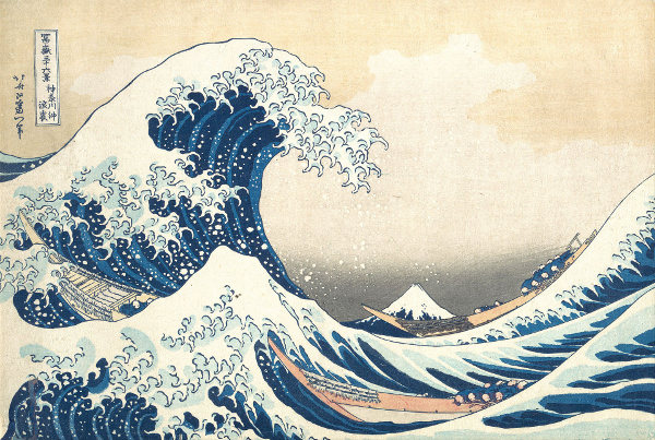
One consequence of nonlinearity is non-uniqueness of a certain kind in the solutions. When a water wave has a huge amplitude (as in a tsunami), the height of the water surface can be a three-valued function of distance along propagation; in this celebrated print, the great Japanese artist Hokusai chose to catch one of his Eighteen Views of Mount Fuji by framing it within a curling wave just before it crashes. Another instance is the flow between two rotating concentric cylinders with fluid in the gap, usually called cylindrical Couette flow. G.I. Taylor, one of the great leaders of fluid dynamics in the 20th century (Figure 5), showed theoretically, and demonstrated experimentally, that there was an instability in this flow involving vortical cells, and there was excellent agreement between his theory and his experiments on the onset of instability (Figure 6). But as we move further away from onset the number of possible flow regimes—defined say by the number of cells and the number of the azimuthal waves that can accompany the cells—can be numerous even at given cylinder speeds, as many as around 25 in [4]. Here is non-uniqueness run riot, so to speak (although, for a given temporal history in rotation speed of the cylinder the end state is unique).

Taylor was a Cambridge mathematician who not only made experiments (as Figure 6 indicates) and solved equations, but also sailed boats and flew airplanes. Fluid dynamics during the 20th century had very porous boundaries. Among the people I learnt most from at Caltech were Hans Liepmann (a physicist by education), Paco Lagerstrom (a mathematician who was working at Douglas Aircraft before Clark Millikan (Robert’s son and Director of the Aero Lab) took him to Caltech) and Anatol Roshko (an engineer).

Let us now look at Nonlinearity, Act I. In the late 19th and early 20th century nonlinearity was still new, and the subject of ‘hydrodynamics’ abounded in ‘paradoxes’. Most of these were considered by Garrett Birkhoff in a book published in 1950¹ (his definition of paradox was that it represented an apparent inconsistency between fact and plausible argument). The subtitle of Birkhoff’s book tells us about the mathematical mystery surrounding fluid flows. The frontispiece to the book showed a supersonic flow with shock waves, which Birkhoff considered at the time an instance of ‘common sense contradicted’, because it involved so many virtually discontinuous solutions. But today such pictures are daily fare for space scientists and missile engineers.

The grand-father of all these paradoxes is the one due to d’Alembert, who in 1768 proved (assuming zero viscosity, among other things) that the drag of a finite body in steady motion was zero. (His ‘proof’ implied that at \nu = 0 the flow should plot at +1 (point K) on the ordinate in Figure 2—i.e., steeply up the scale in the diagram.) Of course we know that drag is not zero in real life, hence the paradox. D’Alembert knew this too, but he left it “to future Geometers for elucidation” (he must have been a Greek at heart, for mathematics meant geometry in classical Greece). The prize that was promised by the Berlin Academy on the subject was not awarded, because they had (wisely) demanded experimental evidence in support of the analytical ‘proof’. (So we can wonder whether mathematics is here seeking to provide the ‘proof’ for the experiment, or experiment to provide the ‘proof’ for the mathematics, but at any rate the Clay Prize of today continues an old fluid-dynamical tradition of problem-solving awards.) This ‘d’Alembert paradox’ was one of the many instances that led to the Hydraulics-Hydrodynamics wars, fought because it was said that the former (created and exploited by engineers) observed things which could not be explained, whereas the latter (pursued by ‘geometers’, i.e. mathematicians) explained things that could not be observed. (The word hydrodynamics was invented by Daniel Bernoulli, who confused the issue by using it as the title of a book he wrote on hydraulics.)

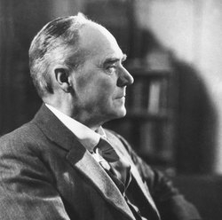
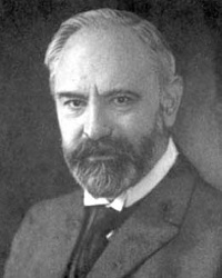
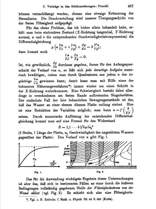
The paradoxes slowly got resolved in the first half of the 20th century, largely through the change in thinking wrought by one man, the German engineer Ludwig Prandtl, who successfully bridged the epistemological gulf with the mathematicians. Prandtl was working in industry when the famous mathematician Felix Klein persuaded him to move to Göttingen as a professor of applied mechanics—surely one of the most inspired appointments ever made in the history of fluid dynamics. In 1904, Prandtl read a paper at the 3rd International Congress of Mathematicianss at Heidelberg (porous borders again!), and introduced a new mathematical method of handling nonlinearity—chiefly in laminar flow problems—by creating the concept of boundary or singular layers—small regions within which the nonlinearity and viscous effects were concentrated and could by clever approximations be managed. This approach yielded interesting asymptotic solutions in the \nu \rightarrow 0 limit. We could in fact truthfully say that this particular page in Prandtl’s paper of 1904 (Figure 7) gave birth to modern fluid dynamics, and resolved d’Alembert’s paradox.

Prandtl’s method was later codified into singular perturbation theory by (among others) the same Friedrichs I had met in Bangalore, and in particular by Paco Lagerstrom, developing what came to be called the method of matched asymptotic expansions (MAX for short). Many paradoxes dissolved under the appropriate MAX attack. One of the most dramatic uses of MAX (not so called at the time) was the demonstration of the instability of Prandtl’s boundary layer by his student Tollmien (1929). It took more than a decade before this instability was observed experimentally, in contrast with Taylor’s almost instantaneously successful comparison of theory and experiment (shown in Figure 6). This led to some controversies between the two leaders in 1938, although each of them respected the other greatly. (G.I. Taylor proposed Prandtl for the Nobel Prize, even calling Prandtl his ‘chief’; but next year their two countries were at war with each other, and the Nobel Prize was forgotten.)

The whole area of hydrodynamic instability has been the joint enterprise of physicists (Sommerfeld, Rayleigh, Heisenberg), mathematicians (Orr, Taylor), engineers (Reynolds, Prandtl, Tollmien, Schubauer) (porous borders again). The subject is important because many flows crumple into some form of instability or other at the slightest excuse, making them prone to turbulence.

But even MAX cannot handle what (Sir) Horace Lamb, in his ever-enduring treatise called

Hydrodynamics that summarised pre-modern fluid dynamics, called ‘the chief outstanding difficulty of our subject’, namely turbulence—the apparently random/irregular/chaotic/intermittent vortical motion that is the natural state of most air and water flows we observe.

It remains to call attention to the chief outstanding difficulty of our subject.
—Sir Horace Lamb in Hydrodynamics, 6th edition (Cambridge University Press, 1932)

That brings us back to turbulence and pipe flow, and how our Indus valley ancestors who pushed water through their cities more than 4000 years ago clearly knew things that as mathematicians we still cannot explain. In nearly 135 years since Reynolds made his famous experiments we have learnt a lot about turbulent flows. For example, engineers can predict not only the pressure loss in a pipe, but also the drag of an aircraft or the trajectory of a satellite launch vehicle with considerable confidence—but not starting from first principles, and not without appealing to experimental data at some stage or the other. All we can say is that a lot of clever analysis has gone into reducing the amount of data that needs to be acquired, but the problem of getting it all from first principles remains unsolved. So the chief outstanding difficulty of Horace Lamb remains just that to this day.

Before I close however I want to show you some flow pictures, for fluid dynamics is nothing if it is not photogenic. (As John Ruskin said, nature produces its most beautiful inorganic forms in water flow.) Prandtl’s path-breaking paper at the International Congress of Mathematicians contained numerous flow pictures at the end. The pictures I now show (following his example) were all taken in Bangalore. The first (Figure 8) shows how flows can be generated in the laboratory to look like clouds in the atmosphere. As the fake clouds are generated in a water tank the great resemblance we see with real clouds shows the extraordinary power of the idea of dynamical similarity: isn’t it amazing that a cloud made by the motion of moist air over a height of several kilometers in the atmosphere can be mimicked in a plume generated in a little water tank that is a cube of about 1 m side—if only we put the right amount of heat at the right place and right time into the laboratory plume?

One of the intriguing things about turbulence is that a flow we consider random or chaotic may actually possess concealed order. This was convincingly demonstrated by Brown and Roshko in the 1970s. Figure 9 shows an instance where the order concealed in a plume can be revealed by its wavelet transform.

I have already mentioned the phenomenon of transitions from laminar to turbulent flow but reverse transitions from turbulent to laminar flow are also possible. Here is one instance (Figure 10) where that happens in a rather dramatic way, by the simple expedient of bending the tube carrying turbulent flow (red, diffused in the picture) into a coil (leading to the green, non-diffusing filament of laminar flow at the third coil). This phenomenon can be seen as the anti of that studied in Reynolds’ experiment.

So the big question is: What is the mathematics that can handle all these phenomena? In a well known lecture given at the Courant Institute, Eugene Wigner once spoke eloquently about the unreasonable effectiveness of mathematics. But for all those who have been collectively wrestling with turbulence for more than a century, what seems striking is the singular ineffectiveness of mathematics in handling the highly nonlinear Navier–Stokes equations (hence the Clay Prize). Fluid flow has always been a complex problem. The Yoga-Vāsiṣţha (6th/7th century?) drew parallels between the richly diverse ways in which water flows and the human mind works. Galileo said he knew more about the motion of heavenly bodies than about the flow of water under his very eyes. Echoing this thought more than three centuries later, Feynman pointed out that we can follow the evolution of a star till convection starts, but thereafter we can no longer deduce what should happen. “A few million years later the star explodes, but we cannot figure out the reason”—thus his conclusion that turbulence was the greatest unsolved problem in classical physics. After writing down his equations in 1757 (basically Navier–Stokes without the viscous terms), Euler declared that the difficulty with fluid flows was not the sufficiency of the principles of mechanics but the fact that “analysis abandons us here”. But the man who saw most clearly the fundamentally mathematical nature of the problem was von Neumann. He thought that if the turbulence problem were solved, its impact on pure mathematics would be even greater than on fluid dynamics (this thought is tucked away in a report he wrote for the US Office of Naval Research that has not been widely read, in part because he thought it was not ready for publication). That is why the greatest advances in fluid dynamics have for long generally depended on deep physical insight, clever experiments, smart approximations, accurate numerical solutions and so on, rather than a grand solution to the central problem.

Simply put, if we know the equations but cannot find their crazy solutions, we must conclude that we need some new mathematics. May be some young person some day will create it! As of now, we are like the blind men and the elephant in the universally famous Buddhist story (Figure 11, with many thanks to Prof. Anatol Roshko for his wonderful cartoon).

Good luck to all those who are still fighting the ‘turbulence problem’ with Fluid Mathematics.

References

• [1] A. Roshko. 1993. Perspectives on Bluff Body Aerodynamics. Journal of Wind Engineering and Industrial Aerodynamics 49.1-3:79–100.
• [2] O. Reynolds. 1883. XXIX. An experimental investigation of the circumstances which determine whether the motion of water shall be direct or sinuous, and of the law of resistance in parallel channels. Phil. Trans. Royal Soc. London 174: 935–982.
• [3] R. Narasimha. 1957. On the Distribution of Intermittence in the Transition Region of a Boundary Layer. Journal of Aeronautical Science. 711–712.
• [4] D. Coles. 1965. Transition in Circular Couette Flow. Journal of Fluid Mechanics. 21(3):385–425.
• [5] G.I. Taylor. 1923. VIII. Stability of a viscous liquid contained between two rotating cylinders. Phil. Trans. Royal Soc. London. Series A, Containing Papers of a Mathematical or Physical Character 223:289–343.
• [6] G.S. Bhat, R. Narasimha, and V. H. Arakeri. 1989. A New Method of Producing Local Enhancement of Buoyancy in Liquid Flows. Experiments in Fluids. 7(2):99–102.
• [7] R. Narasimha, V. Saxena S. and Kailas. 2002. Coherent Structures in Plumes with and without Off-Source Heating Using Wavelet Analysis of Flow Imagery. Experiments in Fluids. 33(1):196–201.
• [8] P.R. Viswanath, R. Narasimha, A. Prabhu. 1978. Visualization of Relaminarizing Flows. Journal of the Indian Institute of Science. 60(3):159–166.

Footnotes

1. G. Birkhoff. Hydrodynamics: A Study in Logic, Fact and Similitude, Princeton, NJ, 1960. ↩