\pi, the all-pervading mathematical constant, has always fascinated mathematicians. Srinivasa Ramanujan was no exception. In 1914, he derived a set of infinite series that seemed to be the fastest way to approximate \pi. However, these series were never employed for this purpose until 1985, when it was used to compute 17 million terms of the continued fraction of \pi. And in the years preceding this computing feat, there were breakthroughs in understanding why Ramanujan’s series approximated \pi so well. This article explores this recently gained understanding of Ramanujan’s series, while also discussing alternative approaches to approximate \pi.
William Shanks, a 19th century amateur British mathematician, had a flair for computation. Aside from having published a table of prime numbers up to 60,000, he computed highly accurate estimates—correct up to 137 decimal places—of the natural logarithms of 2, 3, 5, 7 and 10. However, his most accurate calculation would be that of \pi.
Mathematically, Shanks’ \pi calculation can never end. \pi is not a rational number, which means its decimal expansion is infinite in length, with no repeating pattern. The common rational approximation of \pi, 22/7, has an infinitely long but repeating decimal expansion (3.142857142857\ldots), aside from being incorrect from the third decimal place onwards.
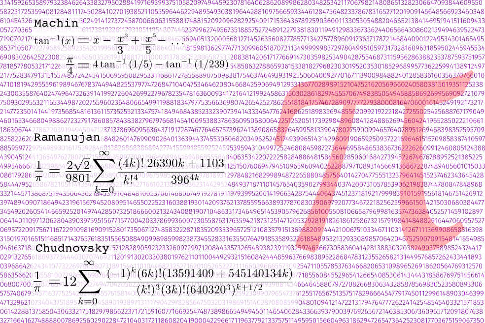
Around 1873, Shanks computed \pi to 707 decimal places, a record at the time, by employing an infinite series discovered by the astronomer John Machin [1],
\frac{\pi}{4} &= 4 \tan^{-1}\left(\frac{1}{5}\right) ~-~ \tan^{-1}\left(\frac{1}{239}\right) \\
&= 4\left(\frac{1}{5}-\frac{1}{3}\left(\frac{1}{5}\right)^3 + \frac{1}{5}\left(\frac{1}{5}\right)^5 – \cdots\right)
– \left(\frac{1}{239}-\frac{1}{3}\left(\frac{1}{239}\right)^3 + \frac{1}{5}\left(\frac{1}{239}\right)^5 – \cdots\right).
\end{alignat*}\]
The above formula involves the sum of an infinite series of terms. The number of terms that need to be evaluated to provide the desired number of digits of \pi is determined by the convergence of the series sum. Convergence refers to the rate of increase in the number of correct digits of a sum as the number of terms evaluated increases.
Machin’s formula converges to \pi at the rate of about one or two digits per term, i.e. calculating an additional term of the series provides one or two extra digits of \pi [2]. Thus, Shanks must have evaluated at least 500 terms of Machin’s formula! Alas, in 1944, it was discovered that Shanks’ calculation was incorrect from the 527th digit onwards [3].
But Shanks wasn’t alone in exploring \pi with an infinite series. A few decades later, a 1914 issue of the Quarterly Journal of Pure and Applied Mathematics would carry one of the world’s first glimpses of what G.H. Hardy had termed as Srinivasa Ramanujan’s “invincible originality” [4]. Ramanujan’s publication, titled “Modular Equations and Approximations to \pi”, contained not one, but seventeen different series that converged so rapidly to \pi that one could match the accuracy of Shanks’ monumental effort despite evaluating far fewer terms.
In the subsequent decades, two developments radically advanced efforts to compute the digits of \pi. First, considerable efforts to understand the methods employed by Ramanujan gave rise to recipes to build series that converged even faster than Ramanujan’s original series expansions. And in parallel to these efforts, the rapid increase in computing power would make it possible to evaluate millions of terms from these series to give enough digits of \pi to populate an entire bookshelf if printed (Figure 1).
The computing has not stopped. In 2013, Alexander Yee, then a graduate student at the University of Illinois at Urbana-Champaign, USA and Shigeru Kondo, an engineer in Japan, went far beyond Shanks’ imagination. Kondo ran a program called y-cruncher, written by Yee, to compute 12.1 trillion digits of \pi, a record at the time for the most number of digits of \pi calculated[5]. Their computation took over 371 days on a self-assembled desktop computer [5].

Feats of \pi digit computation such as these are rarely required for any physical calculation. Indeed, only 39 digits of \pi are required to compute the volume of the known universe to an accuracy of a single atom [6]. But the execution of large computations, such as ones that find digits of \pi, have led to quicker algorithms for multiplying numbers. “I’m more interested in the methods for computing it \pi rather than the actual digits”, says Yee, who specializes in high performance and parallel computing. These computations have also helped spot flaws in computer circuits. In 1986, David Harold Bailey, a mathematician and computer scientist who has co-developed several well known series of \pi, once found a fault in the hardware of a NASA supercomputer while attempting to compute 29 million digits of \pi [6].
But the thrill and motivation to find digits of \pi goes far beyond this for most \pi enthusiasts.
The question of whether patterns exist in the digits of \pi is a question that has possessed many through the ages. “What if I gave you a sequence of a million digits from \pi? Could you tell me the next digit just by looking at the sequence?”, asked Gregory Chudnovsky, now a professor at New York University [9],[10]. This series expansion is quite popular in the \pi computing community. It is, in fact, the same series that was used by Yee and Kondo in 2013 during their 12.1 trillion digit \pi computation.
While the Chudnovskys employed mathematical methods similar to those in Ramanujan’s 1914 paper to derive their series formula for \pi, the terms they derive in their final series are different from those of Ramanujan. The most popular series supplied by Ramanujan in 1914, which gives 8 digits of \pi for every term evaluated, is
\frac{1}{\pi} = \frac{2\sqrt{2}}{99^2}\sum_{k=0}^\infty \frac{(4k)!}{k!^4}\frac{26390k + 1103}{396^{4k}}.
\label{eqn:1overpi}
\end{alignat}\]
Mathematicians have worked out the recipes from which to derive Ramanujan’s series [3]. This article will broadly explore the reasons for the rapid convergence of this series. Mathematicians have worked out the recipes from which to derive Ramanujan’s series [11]. This article will broadly explore the reasons for the rapid convergence of this series.
Our first step is to look at Machin’s formula, the one employed by Shanks in 1873. It involves adding the terms of a series representation of the inverse trigonometric function \tan^{-1}(x). These functions are encountered when one has to compute an angle in a triangle given the lengths of its sides. Other inverse trigonometric functions include those of \sin^{-1}(x) and \sec^{-1}(x). The first known infinite series representations of these functions were computed by Madhava(1340–1425), and also by Gottfried Leibniz(1646–1716) [12]:
\tan^{-1}(x) &= x~-~\frac{x^3}{3} + \frac{x^5}{5}~-~\cdots, \\
\sin^{-1}(x) &= x + \left(\frac{1}{2}\right)\frac{x^3}{3} + \left(\frac{1\cdot3}{2\cdot4}\right)\frac{x^5}{5}+\cdots.
\end{alignat*}\]
Since \tan^{-1}(1) = \pi/4, we can substitute x=1 in the series for \tan^{-1}(x) to compute digits of \pi. Similarly, since \sin^{-1}(1/2)=\pi/6, substituting x = 1/2 in the series for \sin^{-1}(x) gives digits of \pi. However, these series converge more slowly to \pi than Machin’s formula and are rarely used for this purpose.
Amongst his other contributions to mathematics and philosophy, Leibniz is famous for developing integral calculus. Leibniz considered an integral to be solved if a closed form solution, or a formula, could be derived for it. For instance, the integral \int_0^x\cos(x)dx is solved since it is equal to \sin(x). Remarkably, the same inverse trigonometric functions described earlier emerge as solutions to the following integrals
\[\begin{alignat*}{2}
\tan^{-1}(x) &= \int_0^x\frac{dt}{1+t^2}, \\
\sin^{-1}(x) &= \int_0^x\frac{dt}{\sqrt{1-t^2}}.
\end{alignat*}\]
In the search for such closed form representations of integrals, mathematicians encountered some that seemingly evaded solution, such as the elliptic integral of the first kind
\[ \int_0^{\pi/2}\frac{1}{\sqrt{1-k^2\sin^2(u)}}du , \]
which is denoted as K(k), where 0 < k < 1 is a parameter. Eventually, Joseph Liouville (1809-1882) would prove that there exist integrals whose solution cannot be expressed in a closed form in terms of functions such as the trigonometric functions.
The elliptic integral K(k) arises in physics, for instance, when one attempts to compute the time period of a simple pendulum. For a simple pendulum of length \ell, its time period of oscillation, T, is given by
\[\begin{equation}
T = 4\sqrt\frac{\ell}{g}K\left(\sin\left(\frac{\theta_0}{2}\right)\right),
\label{eqn:pendulum-elliptic}
\end{equation}\]
where \theta_0 is the maximum amplitude of oscillation. High-school physics textbooks typically teach that T \approx 2\pi\sqrt{\frac{\ell}{g}}. This value of T is accurate only when \sin\left(\theta_0/2\right) is close to zero, which occurs when \theta_0 is very close to zero. This corresponds to a pendulum that has a very small amplitude of oscillation. Since K(k=0) = \pi/2, and \sin^2\left(\theta_0/2\right) \approx 0 in this case, we get K\left(\sin\left(\theta_0/2\right)\right) \approx K(0) = \pi/2. By substituting this value of K\left(\sin\left(\theta_0/2\right)\right) in \(\eqref{eqn:pendulum-elliptic}\), we get T \approx 2\pi\sqrt{\frac{\ell}{g}}.
This integral is central to the emergence of not only Ramanujan’s many series of 1/\pi, but is also the basis of iterative methods that improve upon a starting “guess” of the value of \pi in a step-wise fashion. They provide an alternate way of finding digits of \pi without having to evaluate terms of an infinite series. Iterative methods of \pi can be loosely thought to work in the following fashion
\textrm{Estimate of } \pi \textrm{ at step #} (n) &= \textrm{Estimate of }\pi\textrm{ at step #} (n-1) + \nonumber \\
&\textrm{(or)}\times\textrm{term to reduce error of estimate at step #} (n-1).
\label{eqn:general-iterations}
\end{alignat}\]
This brings us to the iterative method known as the arithmetic-geometric mean (AGM), proposed by Carl Friedrich Gauss (1777–1855) [11]. In the AGM, one starts with two numbers a_0 and b_0, and computes, or iterates, successive values a_0,a_1,a_2,\ldots and b_0,b_1,b_2,\ldots by the following rule
\[
a_{n+1} = \frac{a_n+b_n}{2}\,\,,\,\,b_{n+1}=\sqrt{a_nb_n}
\]
In 1975, Richard Brent and Eugene Salamin independently developed an iterative method to compute \pi by using an AGM iteration starting with values a_0=1 and b_0=1/\sqrt{2} [13]. Below are the first four iterations of the Brent-Salamin formula, where only the correct decimal places are shown
\[\begin{alignat*}{2}
\pi_0 = 2.&9142\ldots \\
\pi_1 = 3.&14\ldots \\
\pi_2 = 3.&1415926\ldots \\
\pi_3 = 3.&141592653589793238\ldots \\
\pi_4 = 3.&141592653589793238\\
& 4626433832795028841971\ldots
\end{alignat*}\]
The value of \pi_4 is correct up to 41 places after 4 iterations. The next iterated value, \pi_5, is correct up to 84 places. In fact, it can be shown that the number of correct decimal places of \pi obtained by this method roughly doubles at each iteration, i.e. \pi_n is correct to roughly 2^n decimal places. This is a very rapid rate of convergence, referred to as quadratic convergence. In comparison, obtaining 84 places of \pi through Machin’s formula requires us to evaluate 70 terms of the \tan^{-1}(x) series.
Much of the theory explaining the convergence of methods that iteratively calculate \pi, like the Brent–Salamin Formula, has been worked out by the Borwein brothers, Jonathan and David [11]. Their theory not only provides a recipe for creating iterative schemes that can outrun the Brent–Salamin Formula in reaching \pi, but also shines light on the convergence of Ramanujan’s collection of series.
The Borweins’ recipe consists of two vital ingredients—singular moduli and multipliers. The parameter k in the elliptic integral K(k) is referred to as the integral’s modulus. One evaluates the integral by substituting different values of the modulus. For instance, K(k=0) = \pi/2 . Each modulus has an associated complementary modulus k' of K(k) defined by k' = \sqrt{1-k^2}. The elliptic integral evaluated at k' is either represented as K'(k) or K(k'), and is referred to as the complementary elliptic integral.
Recall that Liouville had proved that it is not possible to write a formula that gives us the value of the integral K(k) for all values of k. There are, however, certain special values of the modulus k for which this is possible. For example,
\[
K\left(k=\frac{1}{\sqrt{2}}\right) = \frac{C}{4\sqrt{\pi}}
\]
where C = 13.145\ldots is a constant. But this isn’t the most surprising property of K(k) evaluated at k=1/\sqrt{2}. At this modulus, K'(1/\sqrt{2})/K(1/\sqrt{2}) = 1. There are an infinite number of such moduli, called singular moduli, where K'(k_n)/K(k_n) = \sqrt{n} when n is an integer [14]. Some singular values are shown in Table 1.
| k_n | K'(k)/K(k) |
|---|---|
| k_2 = \sqrt{2} - 1 = 0.4142\ldots | \sqrt{2} |
| k_3 = (-1 + \sqrt{3})/2\sqrt{2} = 0.2588\ldots | \sqrt{3} |
| k_4 = 3 - 2\sqrt{2} = 0.1715\ldots | \sqrt{4} = 2 |
| ⋮ | ⋮ |
| \(k_{16} = (-1 + \sqrt[\leftroot{0}\uproot{-1}4]{2})^4(3 + 2\sqrt{2}) = 0.0074\ldots\) | \sqrt{16} = 4 |
| ⋮ | ⋮ |
Table 1 : Singular moduli of the elliptic integral K(k) [15]
The second ingredient for building an iterative method is the notion of multipliers between two different moduli that are related by a modular equation. To explore these two ideas, consider the relation
\[\begin{alignat*}{2}
K(k) &= \frac{1}{1+k}K\left(\frac{2\sqrt{k}}{1+k}\right) \\[0.5ex]
&= M_2(l,k)K(l),
\end{alignat*}\]
where l = 2\sqrt{k}/(1+k). Squaring both sides of this equation gives us l^2(1 + k)^2 - 4k = 0. Equations of this form, which relate the two different moduli k and l, are called modular equations. The above relation defines a second order, or quadratic, modular equation. The quantity M_2(l,k) = K(k)/K(l) is the multiplier of order 2 between k and l, since it corresponds to moduli that are related by a quadratic equation. In general, the multiplier of p^{th} order is M_p(l,k)=K(k)/K(l), where k and l are related by a p^{th} degree modular equation.
We now have all the ingredients of the Borweins’ recipe to build an iterative method to calculate \pi. To illustrate a method from this recipe, consider the iterative rule which involves a function \alpha defined as follows
\[\begin{alignat}{2}
l_{n+1} &= \frac{1-\sqrt{1-l_n^2}}{1+\sqrt{1-l_n^2}},\label{eqn:borwein_quad_moduli}\\[0.5ex]
\alpha_{n+1} &= (1 + l_{n+1})^2\alpha_n ~-~ 2^{n+1}\sqrt{r}l_{n+1},\label{eqn:borwein_quad_alpha}
\end{alignat}\]
where, l_n denotes the singular modulus computed at the n^{th} iteration. r is a positive integer whose choice is not relevant here. The modular equation \(\eqref{eqn:borwein_quad_moduli}\) is derived from a quadratic equation, which is why the square of the reciprocal of the 2^{nd} order multiplier M_2(l_n,l_{n+1}) = 1/(1+l_{n+1}) pre-multiplies \alpha_n in \(\eqref{eqn:borwein_quad_alpha}\).In general, if a p^{th} order modular equation is used in deriving \(\eqref{eqn:borwein_quad_moduli}\), then 1/M_p^2(l_n,l_{n+1}) pre-multiplies \alpha_n in \(\eqref{eqn:borwein_quad_alpha}\).
If we start iterating this method with l_0 = k_1 = 1/\sqrt{2}, we obtain l_1 = k_4 \approx 0.1715, l_2 = k_{16} \approx 0.0074, and so on, with these moduli ultimately reaching zero, as can be seen in Table 1. At the same time \alpha_1,\alpha_2,… converge quadratically to 1/\pi.
The quadratic convergence of equations \(\eqref{eqn:borwein_quad_moduli}\), \(\eqref{eqn:borwein_quad_alpha}\) is because l_{n+1} is calculated from l_n using a quadratic modular equation. Convergence to 1/\pi is accelerated if a higher order modular equation is used to derive \(\eqref{eqn:borwein_quad_moduli}\). As the order of the modular equation used is increased, the iterations jump between moduli that are farther away than when a lower order equation is used. This means that the moduli are more quickly declining to zero. In the general scheme of iterative methods like \(\eqref{eqn:general-iterations}\), this leads to a quicker correction of errors at each step.
Imagine the iterative process of computing 1/\pi as crossing a river starting at one bank (the initial value) by jumping between rocks placed in the river (the singular moduli) to reach the other bank (1/\pi). Iterations with a p^{th} order modular equation is much like jumping from one rock to the p^{th} rock, instead of merely stepping from one rock to the immediate next one. This means that one crosses (converges) faster to the other bank.
Each term of Ramanujan’s 1/\pi series in \(\eqref{eqn:1overpi}\) can be written in terms of the rapidly converging \alpha functions defined by the Borweins in \(\eqref{eqn:borwein_quad_alpha}\). Most remarkably, these terms contain singular moduli and multipliers obtained from a 58^{th} order modular equation [3]. While techniques to evaluate such higher order singular moduli have been developed today, this is perhaps yet another reminder of the immense arsenal of computational techniques that Ramanujan had at his command.
In comparison to the iterative methods that seem to gallop towards \pi, Ramanujan’s series appear to converge far more slowly, with each term providing only 8 correct decimal places of \pi. In reality, however, the iterative methods are a lot slower to run on computers compared to series methods. “In practice, the Chudnovsky formula is more than 3 times faster than AGM methods”, says Yee.
Some multi-million digit \pi computations carried out in the early 1980s used iterative methods like the Brent–Salamin Formula despite their relatively slower speed [3]. For reasons yet unclear, Ramanujan’s collection of series were rarely used in \pi computations. That all changed in 1985 when Ralph William Gosper, a computer scientist and mathematician, went on a record-setting voyage through the digits of \pi using Ramanujan’s 1/\pi series.
“I first saw the Ramanujan series while an undergraduate, in The World of Mathematics books. I was so envious of Ramanujan’s results…”, recalls Gosper. He was then a student at the Massachussetts Institute of Technology (MIT), working toward a Bachelor’s degree in mathematics. One of Gosper’s research interests include the study of continued fraction representations of real numbers. These are representations of the form
\[x = a_0 + \cfrac{b_1}{a_1 + \cfrac{b_2}{a_2 + \cfrac{b_3}{a_3 + \ldots}}} \]
where a_0,a_1,a_2,\ldots and b_0,b_1,b_2,\ldots are integers. Such a representation is a simple continued fraction if each of b_0,b_1,b_2\ldots are equal to one. In this case, the simple continued fraction can be concisely represented as [a_0;a_1,a_2,\ldots]. If x is rational, the number of continued fraction terms is finite; but if x is irrational, like in the case of \pi, the number of fractional terms is infinite. The first hundred terms of the simple continued fraction of \pi are shown in Figure 2.
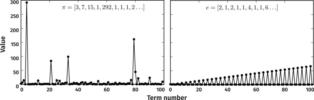
Gosper utilized Ramanujan’s 1/\pi series \(\eqref{eqn:1overpi}\) to not only compute digits of \pi but also to find as many terms of its continued fraction representation as he could. Unlike the Chudnovskys, who focussed on patterns in the decimal expansion of \pi, Gosper looked for patterns in the continued fraction. “If you can prove that the absence of patterns persists, you settle the age-old question of the irrationality of \pi+e, \pi e, \pi/e, etc.”, says Gosper. Here, e refers to the irrational number that is the base of the natural logarithm, which arises in many mathematical and physical problems. Even today, it is unknown if the sum, product and quotient of e with \pi are irrational. e seems different from \pi in that the terms of its simple continued fraction display a clear pattern compared to those of \pi (Figure 2).
Gosper computed over 17 million digits of \pi, a record at the time, as well as a little more than 17 million terms in the continued fraction of \pi [3]. He also found the largest term known in the simple continued fraction of \pi (878783625) which is the 11,504,931^{th} term. While his \pi digit record was short-lived, his record for the largest continued fraction term computed stood for over a decade. He fondly remembers this computation as he encountered his “lifetime’s most terrifying bug”. Had he not routinely checked his computation at intermediate stages, he might have shared in the bad luck of William Shanks. “My \pi would have been wrong and I’d have been clueless”, he says.
This wasn’t the only twist in the tale of Gosper’s computation. When he ran his program, there was no proof at the time that Ramanujan’s 1/\pi series actually converged to 1/\pi. He reportedly had to compare the first 10 million digits with an earlier \pi digit calculation. This verification was also the first preliminary proof that Ramanujan’s series actually converged to \pi [3].
The years since 1985 have seen multiple publications propose and study generalizations of Ramanujan’s 1/\pi series. In 2007, one such paper titled “Ramanujan-type formulae for 1/\pi : A second wind?” was uploaded to the Internet by Wadim Zudilin, a Russian number theorist [16]. The author intended to “…survey the methods of proofs of Ramanujan’s formulae and indicate recently discovered generalizations, some of which are not yet proven.” And on Pi Day 2016, celebrated each year on March 14 (since the date can be written as 3/14), Alexander Yee released more software from his work on y-cruncher that allows other \pi enthusiasts to go (decimal) places with \pi.
Evidently, even more digits of \pi lie within our computational grasp while mathematicians still find new ripples from the splash created by Ramanujan’s paper over a hundred years ago.
References
- [1] Shanks, William in Complete Dictionary of Scientific Biography. Online; accessed 23 March 2016.
- [2] R.E. Schwartz, Machin’s Method of Computing the Digits of \pi. Online; accessed 23 March 2016.
- [3] J.M. Borwein, P.B. Borwein and D.H. Bailey, Ramanujan, modular equations, and approximations to pi or how to compute one billion digits of pi. The American Mathematical Monthly, 96.4 (1989), pp. 20–219.
- [4] S. Ramanujan, Modular equations and approximations to \pi, Quarterly Journal of Pure and Applied Mathematics, 45, pp. 350–372.
- [5] A. Yee, Round 2… 10 Trillion Digits of Pi. Online; accessed 23 March 2016.
- [6] J. Arndt and C. Haenel, Pi unleashed, Springer Science & Business Media (2001).
- [7] Did you ever wonder… why the digits of \pi look random?. Online; accessed 23 March 2016.
- [8] R. Preston, The mountains of Pi, The New Yorker 2 (1992), pp. 36–67.
- [9] A. López-Ortiz, How to compute digits of pi?. Online; accessed 24 March 2016.
- [10] D.V. Chudnovsky and G.V. Chudnovsky, The computation of classical constants, Proceedings of the National Academy of Sciences of the United States of America 86.21, pp. 8178–8182.
- [11] J.M. Borwein and P.B. Borwein, Pi and the AGM, Wiley, New York, 1987.
- [12] I.G. Pearce, Madhava of Sangamagrama, MacTutor History of Mathematics archive 2002.
- [13] E.W. Weisstein, Brent-Salamin Formula. Mathworld – A Wolfram Web Resource. Online; accessed 23 March 2016.
- [14]E.W. Weisstein, Elliptic Integral Singular Value. Mathworld – A Wolfram Web Resource. Online; accessed 23 March 2016.
- [15] V.V. Petrović, Comprehensive Table of Singular Moduli. Online; accessed 26 March 2016.
- [16] Wadim Zudilin, Ramanujan-type formulae for 1/\pi : A second wind?. Online; accessed 23 March 2016.