
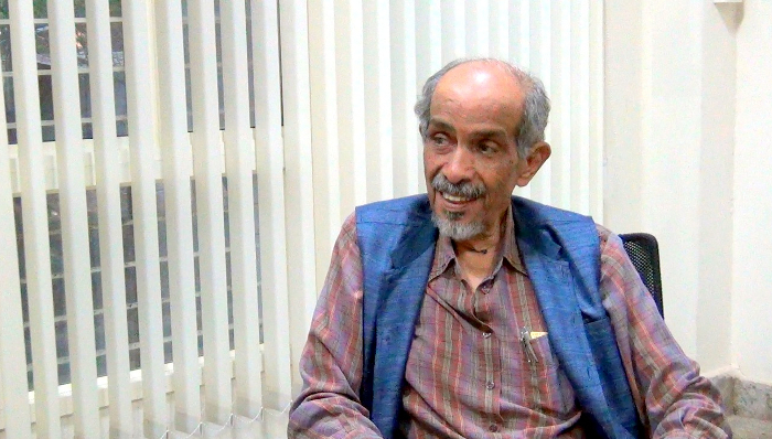
Roddam Narasimha, popularly known as RN, is a multifaceted scientist whose academic career has almost entirely been in India, particularly in Bengaluru. He represents a rare combination of a person completely at ease with both the Eastern and Western systems of doing science. He has been at the helm of several indigenous projects instrumental in placing India as an able scientific power. In recognition of his services, he was awarded the Padma Vibhushan, India’s second highest civilian honour, in 2013. Presently, he is DST Year-of-Science Professor at the Jawaharlal Nehru Centre for Advanced Scientific Research, Bengaluru.
The first part of this interview appeared in the April 2017 issue of Bhāvanā. RN spoke to the contributing editors of Bhāvanā in July 2017 for this second and final part of the interview.
Arrival at Caltech and the Launch of Sputnik
On behalf of Team Bhāvanā, thank you for making the time to join us today.
RN: Pleasure.
In the earlier part of your interview for our April 2017 issue, we went over your upbringing in Bengaluru and some of your thoughts on ancient Indian science. Today we would like to talk about your time at the California Institute of Technology [Caltech], and your research interests after you came back to IISc.
So, you started your PhD in 1957?
RN: That’s right.
1957 was also the year that Sputnik was launched. What was the atmosphere in Caltech like at the time? This was the beginning of what would go on to be called the space race. Did this impact the kind of research that took place there, and around California during your PhD?
RN: Yes, I think it had a profound impact on the United States. In fact, the launch of the Sputnik happened within a week of my registration for my PhD. [Laughs] I went there thinking I would work on turbulent flows. And in fact, the first problem I did had to do with the related subject of aerodynamic noise. One problem at that time was that jet engines were making too much noise, and it was a very active area, both as a scientific as well as a technology problem.
However, the fact that the Russians had actually launched a satellite, before the United States did, had a profound effect on the Americans. I still remember that when the Russians announced the launch of Sputnik, very few people believed it. The Russians said that you can hear a beep on a particular frequency, which they said would decisively prove that the satellite was there. But many Americans said that you get beeps from anywhere and we don’t know if it’s coming from the satellite. So finally the Russians announced when exactly Sputnik would appear over the horizon in different cities. For example, it said it would appear in Los Angeles on the western horizon at some time like 6:35 pm on a certain day.
I remember the day very well when everyone at Caltech, from the president of Caltech to the janitors, so to speak, were there wondering if they would be able to see that bright little thing moving in the sky. All the terraces were occupied, and people were there everywhere. Then, precisely at the announced time, it promptly came over the horizon. Its velocity was sufficient to perceive its motion, not very fast since it was far away.
So you could actually see Sputnik, and then everything changed overnight in the United States. The Americans were sure now that the Russians had actually done it. The same experience would have been repeated in other places. It was a turning point as it was seen as a national challenge to the United States. Therefore, they very quickly organized themselves to start a space programme.
One of the other things that impressed me was how quickly those changes were made, and in fact they made steep cuts in the budget for aeronautics research programmes. So the huge budget that the aeronautics programme used to receive was cut down drastically, and a lot of it was spent towards getting ready for space. The research programme in various departments changed, and many aeronautics departments became departments of astronautics and aeronautics, and they started looking at new problems.
You could actually see Sputnik, and then everything changed overnight in the United States
Now, I did the problem on jet noise and I actually worked with a visitor from MIT, Professor Erik L. Mollo-Christensen, as well as with my advisor Hans Liepmann. We finished that work and submitted it for publication—it was published in the Journal of Fluid Mechanics.1 As far as my advisor was concerned, he was willing to take it as my thesis. I spent probably a year and a half on it. However, within that short time, I had not really learnt whatever I had come to Caltech to learn. I wanted to do something else which could not be too easily done in India.
The problem of jet noise was an interesting problem to work on but it was not sufficiently challenging. So I was quite surprised when Liepmann said, “You know, if you want to get your degree, you can write your thesis on it. And then stay here as a postdoc.” But I said, “Well, I think that I need to do some more and I need to learn something more.” And at that time, he was beginning to work on low-density gas dynamics. This was one of the effects of the advent of space.
Satellites usually are hundreds of kilometres up in the sky, and the ordinary Navier–Stokes equations don’t apply there. The Boltzmann equation is what you have to solve in this case, so everybody suddenly got interested in this equation. There were always some people who had been working on it on the side, and so it was not entirely new, but the emphasis on it increased remarkably fast.
My advisor, Hans Liepmann, was actually a physicist by training and, for him, the Boltzmann equation was not new. He instead saw this as an opportunity to do something which really came directly from his training—and by the way, one of his gurus in Germany, Edgar Meyer, had even been a student of Ludwig Boltzmann.
So Liepmann decided to set up a research programme in rarefied gas dynamics, and I said I would like to work on that subject. He was actually making a series of measurements on flow through an orifice, which covered the whole range from where Navier–Stokes and Euler equations are valid, all the way to when they are totally invalid. He could cover the whole range in a small apparatus—it was a physicist’s experiment. [Laughs]
So he made these measurements and got all those results in the continuum regime, which agreed with Euler’s theory. At the other extreme limit, it agreed with what Martin Knudsen, a Danish scientist, had predicted. But in between, it was all new and could not be treated by any known theory. So I offered to make an attempt to see if I could do something toward the free-molecule end of the continuum—a nearly free molecule regime.
Those were still early days for computing. There was a computer at Caltech, but it was not in much use. In fact, some of the senior faculty in Caltech did not particularly approve of using computers because they considered that our analytical skills would go down. [Laughs]
Rarefied Gas Dynamics and the Boltzmann Equation
Was Paco Lagerstrom there at Caltech at the time?
RN: Yes. Lagerstrom was really very strong in analytical thinking. He was one of the people who felt that with the advent of computing, one’s powers of analysis might go down and people will gradually forget how to get useful analytical results. They were actually not wrong. It has actually happened. I mean, fewer people now do the kind of analysis that was being done in the 1950s and ‘60s. While analysis itself may have progressed, many people now, if they can compute, probably will avoid the analysis. Certainly the engineers would—if you could get the result more easily by computing, what’s the use of the approximate method? The approximate methods I learnt as a student in aeronautics are in very little use now. [Laughs] Many of those answers can now be obtained by pushing a button.
Fewer people now do the kind of analysis that was being done in the 1950s and ‘60s
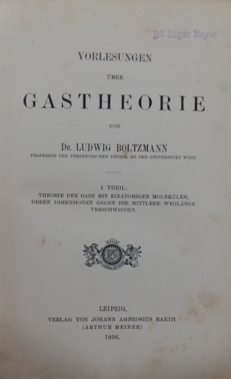
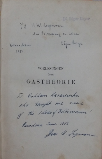
The copy of Boltzmann’s book, Vorlesungen Über Gastheorie, that was passed down from Edgar Meyer to Hans Liepmann to RN Roddam Narasimha
Those years at Caltech marked the beginning of the computing era. But I did a traditional approximate calculation about those nearly free-molecule flows, and it seemed to me that I was making the right assumptions and so on. By the way, the calculation used the BGK (Bhatnagar, Gross and Krook) model—the same Bhatnagar who had set up the Applied Mathematics department at IISc by the time I returned to India. I went ahead and told Liepmann that that’s what I would like to do for my thesis. He said, “Okay, go ahead!” And that’s what I did. That was also an interesting exercise and I published it too.2 But looking back, I think I underestimated the significance of this work and I did not go through in great detail all the assumptions I had made. When I did a calculation and got a result that agreed with the measurements, it then seemed enough. So I published a note.
I later found that there was an international rarefied gas dynamics meeting that very year, but I had not submitted any paper there. I went there just to see how it was going on. I was not even registered, and I go to this lecture hall and this big senior man there is telling the audience, to my horror, that Narasimha was wrong. [Laughs]
Was this happening in Caltech?
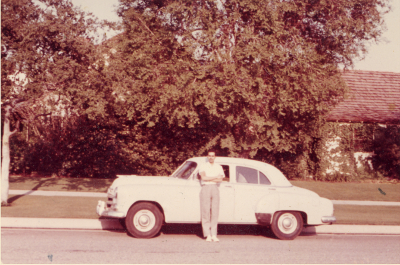
RN: Not in Caltech. It was happening in Berkeley. I went to Berkeley to attend it just for myself. I had by then a car.
I was actually devastated. So I drove back immediately [laughs], and told Liepmann that so-and-so says that my calculations are wrong. And he said, “Well, do you think he’s right?” I said, “No, he is not right. He has not understood the approximation that I have considered.” My advisor said, “Well, you’ve done a piece of mathematics. Now, go and discuss it with the mathematicians in the department.” The department had two mathematicians—Paco Lagerstrom and Julian Cole. I talked to both of them and after a fair deal of discussion, both of them certified that what I had done was sensible. So I had two allies now, who were good and reputed mathematicians.
The speaker in Berkeley came down to Caltech a few weeks later, and we had a long discussion in detail about it. The fact that I had two allies on my side who knew the mathematics, and coupled with my explanation of the mathematics to him, made him have second thoughts about the issue, and he fortunately withdrew his paper. The fact was that, after my note had appeared, he had made some little calculation and found that he got a different answer. Anyway, that taught me a lesson and a longer paper was written later on.3 My confidence in being able to tackle the Boltzmann equation went up because I saw nobody had done that calculation before.
Was this what got you on the map in terms of being consulted by companies?
RN: Yes, perhaps, but there was also the Sputnik effect, which led quickly to the setting up of a large number of private companies. They would get contracts from NASA on problems of physics which NASA had not encountered before.
So they were like the startups of that era?
RN: Exactly. They were the startups of the era, and they were usually run by physicists.
Do any of these still remain?
RN: Mostly, no. But NASA’s programme expanded a great deal and a few of those companies actually became quite big, but the one which caught hold of me to advise them was set up by a physicist.
I worked a lot on rarefied gas dynamics, and enjoyed doing it
By the way, one of those papers I mentioned had to do with another subject connected with the Boltzmann equation, which was a pure piece of mathematics. It showed that in a free molecule flow, under certain conditions, you would have constitutive relations of the Navier–Stokes type. That was actually very funny because in what little I had learned, a free molecule flow is totally different from a continuum flow, and we have to take the molecules into account. But if you make a cloud expand into a vacuum, it so happens that, by a combination of circumstances, the resulting flow behaves as if it is a continuous medium with a viscosity and a conductivity, both of which, however, are time-dependent. Thus, it is not a property of the gas, but it depends on the time that has elapsed since its expansion began.
Coming back to my consultancy, around this time, the chairman of a new company called me. I also mentioned to him what I was doing, and he was very interested. I sent him a preliminary script which was enough for him to hire me, even as I was a student, because there were not too many people working on the Boltzmann equation at that time. A paper was published before long.4
I finally put all these things together, and submitted my thesis and got the degree.5 But JPL [Jet Propulsion Laboratory], which is a NASA lab, got into space research and they were also very interested in this work. Just as I was a consultant to this company, there was also a scientist from JPL who came to me. In my thesis I had said—as I was sufficiently confident—that we could now solve the BGK model to understand the structure of a shockwave, but it would have to be done on a computer.
This was one of the big problems at the time, for a shockwave was commonly thought of as a discontinuity. It actually is not, as it has a non-zero thickness and so it can’t be a discontinuity in reality, but it is very thin, being of the order of the mean free path. That means you really have to work with the Boltzmann equation—you can’t use the Navier–Stokes equations. Navier–Stokes solutions are available, but they can’t be correct for strong shocks.
The Structure of Shockwaves
What are the situations that would give rise to such a shockwave? Are you talking about supersonic flight, or are there other examples as well?
RN: Yes, there was much talk about supersonic flight, but you have shocks on launch vehicles and satellites too. If you have an aircraft flying at supersonic Mach numbers, it is accompanied by a shockwave at the leading edge of the wing and around the nose. There may be more shocks elsewhere too.
Didn’t Charles Yeager achieve supersonic flight in 1947?
RN: That’s correct. It was known that supersonic flight was possible and that the plane would not crash or anything like that. He was the first man to break the sound barrier. But still, the number of people who really understood supersonic flows was at that time not very large. By the time I went to the US, it was a standard degree course. But it was still a new subject; the Boltzmann equation was even newer.
There had been arguments about what happens inside the shockwave, and how you use the Boltzmann equation. Computers had just then come in, and I thought that a good problem would be to try to make a numerical simulation of the Boltzmann equation, and see what it says about the shock structure. My thesis had somehow reached JPL and somebody had seen it, and this man came and said, “You have made this suggestion. Just now I have gotten the first big IBM computer.” I’ve forgotten now what computer it was, I think it was the IBM 350 or so—the biggest computer of the time and the fastest if you wanted the results for the space programme. And JPL was one of the first to get it. So he came and said, “How about doing the shock structure problem on our new computer?”
Liepmann approved it. In fact, Liepmann was the one who had sent him to me. So the work was actually done on the computer and we had solutions. These solutions were once again of the BGK equations. Once again, it gave you an idea of what happens, but the computers were not yet sufficiently powerful to solve the true Boltzmann equation directly.
To come back to your question, yes, the launch of Sputnik changed my programme. I worked a lot on rarefied gas dynamics, and enjoyed doing it.
These lines of work that got opened up on rarefied gas dynamics, were you able to pursue them when you joined IISc as a faculty member? Because you mentioned that to do these numerical simulations at the time, one required the latest computers.
RN: That’s right.
And I imagine that it was something hard to come by at IISc at the time.
RN: Yeah, IISc did not have computers at the time.
Transition from Caltech to IISc
So were you able to carry these interests forward? Because one thing which we have learnt is that you did have a flair for picking problems that were solvable based on the resources that were available to you. Was that something you picked up working with Satish Dhawan?
RN: Well, two things happened. When I came here, we didn’t have a computer and I wasn’t able to do the same things that I did in the United States. But there were a lot of problems in rarefied gas dynamics, some of which were theoretical. There was a problem which I had started working on there in Caltech, that I had not been able to complete. Once again, a piece of mathematics!6 [Laughs] So I continued to work on that. But I also decided, as you said, that while we try to do things which are not being done elsewhere, while still making the best use of what we have, we should also pick problems which are doable. Now the reason that I put it to myself that way is that if you start working on a problem which the Americans are doing, which of course many people here do, well, you are competing with them, without having access to the facilities that they have.
By then I had also learnt a lesson for myself, so to speak—that there are a lot of problems which are interesting and important and actually waiting to be done, but don’t quite get the attention that they deserve, in the United States, for a variety of reasons. That’s the main lesson I learnt from two years of doing research with Dhawan—that there are problems that need to be tackled, crying out to be tackled, and that there is a good chance that you can do it right here in India. So you pick those problems. You can’t say, “Well, Caltech is doing it there, so I’ll also do it here.” But if you knew what Caltech isn’t doing—but could have been doing—then you could do that here.
I told you this story already the last time—that when I left Caltech, they thought that I wouldn’t go back to India. They couldn’t imagine that I could come back to India and not work on the problems that I worked on while at Caltech. But I had made up my mind in any case. So I came back, but as I had not completed that theoretical problem, I actually did go back within six months; because they said, “Well, you know your problem is not complete. We invite you to come here and spend two or three months in the summer” and finish that problem. So I actually went back, not to stay there permanently, but just for the summer. So the problem was being done partly in Caltech and partly in Bangalore, and there were experiments they were doing. I took part a little in that.
But in the Institute [IISc] also, there were interesting things that were going on. I knew what the Institute had been doing. Then I came back once again and picked up problems which you could do here. Some of them were problems which had been suggested by earlier work here, and some others had come up during the six-seven years that I was away.
I decided to work on turbulent flows. Transitions were what I had done during my two years with Dhawan. One of these problems was relaminarization. Flows usually go from laminar to turbulent and the general impression at that time was that once it goes turbulent, it can’t go back to being laminar. But there were experiments in the 1950s in the US and UK which provided some evidence that turbulent flows might be going back to laminar under certain circumstances. For some reason, this did not attract much attention in the United States, perhaps because the evidence was scanty, and not sufficiently convincing.
When I came back in 1962, I found it was a fascinating but neglected problem, so I started a programme to study this. Some thinking had already been done here on this problem, and it eventually became a major project. Some of the first experiments to study it were made here, as was the first real theory, which I think has stood the test of time. It was the subject of K.R. Sreenivasan’s (KRS) thesis.
Relaminarization of Turbulent Flows
His thesis was on the relaminarization of turbulent flows?
RN: It was on the relaminarization of a turbulent boundary layer in particular. And I think it was a very nice piece of work.
Sreenivasan was one of our brightest students. He came with an outstanding academic record, having topped everywhere—he later topped in the Institute too. He came and told me, “I want to do my PhD here.” At the time, I was interested in two subjects—relaminarization and the Boltzmann equation. KRS was interested in both and started on both! So we had Shyam Manohar Deshpande also as an advisor. Deshpande’s thesis had been on shock structure—not with the BGK model, but the full Boltzmann equation.
We quickly found ourselves making a lot of progress on relaminarization. It was actually more interesting because it had not attracted the attention that it deserved. The US was giving a lot more attention to the Boltzmann equation.
Sreenivasan was one of our brightest students
Presumably because of the priorities of the space programme.
RN: Exactly. Some early measurements in relaminarization had been made by M.A. Badrinarayan, one of my colleagues at IISc. And he had a student who made some measurements. Nobody knew exactly what was happening in these flows, and there was no physical model for it. And this is what Sreenivasan’s thesis provided. It worked very well as far as we could see from the scanty data we had at that time from the experiments here, and from another series of experiments by Leslie Kovasznay from the US, just before we had this theory.
So we tried to explain these experimental observations too, and showed that our model could make predictions which were of value. We found out that there were some situations where we couldn’t predict what was happening, but the rest of it was under control, and we could actually say what exactly happens. And that made an impression. Anyway, at that time, that was the only theory available.
It took some years for people to see that there was something to our model. So Sreenivasan and I wrote that paper7 and after a while, we wrote a review in 1979, and showed that there are many other conditions under which relaminarization could happen.
But Kolmogorov tells us that you always expect a flow to go from laminar to turbulent, and it never looks back, and finally dissipates away. In the light of Kolmogorov’s thesis, how does one view relaminarization?
RN: Well, let me put it this way. While it is true that most people generally think only of laminar flows going turbulent, the turbulent-to-laminar reverse transition does not necessarily occur by itself. It usually occurs through an agent which you would not have suspected to have that effect.
Let me tell you one instance where neither Kolmogorov nor Reynolds would have been proved wrong. Let’s say you have a flow. Suppose you take a pipe and the flow is coming in turbulent. Now, start to expand the diameter of the pipe. The velocity of the flow will start to go down. But if the velocity goes down more quickly than the diameter goes up, the Reynolds number will go down. So this pipe grows into this bigger thing where velocity, keeping mass conservation, will go down and the Reynolds number will go down. If the Reynolds number goes below the critical value, it will be laminar. Neither Reynolds nor Kolmogorov would have been surprised here.
However, relaminarization was observed even under circumstances where you would not normally have suspected that it would happen, namely, when you accelerate the flow. In contrast, in the just cited example above with the pipe, the flow decelerates.
You take a boundary layer—it is moving under a certain velocity—and you increase the speed; say, double it or triple it. Then, the boundary layer no longer behaves the way the turbulent boundary layer was expected to behave when accelerated.
Is this regardless of the Reynolds number? At very high Reynolds number too?
RN: That’s the key. Even at high Reynolds numbers. Now, I told you that one of my colleagues did these experiments. He came to a conclusion which I could not actually believe, which was that when you accelerate the flow, the Reynolds number becomes so low that it goes below critical, and so the flow transitions back to being laminar.
Well, that would be the standard logical explanation from what we had learned about Reynolds numbers and so on. But there was Kovasznay’s paper which came just as we were putting the finishing touches on ours, reporting relaminarization at a definitely higher Reynolds number, and where the flow had not gone below the “critical” Reynolds number, but it had already begun to behave differently. So, in fact, the problem that we had set ourselves to solve was: How was it that the flow was laminar, even when the Reynolds numbers are higher than a so-called critical value?
Now, what does it mean for the flow to go laminar? If you start from the fundamentals, and define what you mean by a laminar flow, the ordinary definition would have been: You put a probe in the flow which measures velocity fluctuations; if the velocity fluctuations are random, it is turbulent. But that is too simplistic, because there can be passive turbulent fluctuations, that is to say, you will observe fluctuations, but these don’t determine the dynamics at all.
What we found out in relaminarized flows was that there remained a little bit of turbulence—not as much as you would expect—but it had no effect on the flow. If I incorporated the model without the turbulence terms in the Reynolds equations, it fits the data. So, these were all concepts which were very new then, and one by one, these things were all taken care of. We could eventually explain almost everything.
You asked the question about high Reynolds numbers. Relaminarization has been found on aircraft wings at very high Reynolds numbers. And after we wrote our review in 1979,8 by the 1990s, it looked like interest in relaminarization had declined. We also started doing more work on clouds and direct numerical simulations.
But the high Reynolds number thing had not been settled conclusively. People had seen that fluctuations go down on swept wings. Boeing found that out on the wings of the 737, but nobody knew how to explain it. By this time, people were also building better instrumentation such as laser particle imaging velocimetry and so on. So in the last 15 years, there has been a resurgence of interest in relaminarization at higher Reynolds numbers. The highest now that has been achieved is 5000, based on the momentum thickness, which would be about 100,000 based on the boundary layer thickness, and that would be another order of magnitude greater based on the length. So this is a pretty high Reynolds number.
Relaminarization is happening all the time in our own bodies, literally under our noses
There was also this work of Fernholz and Warnack in Germany who did some high Reynolds number experiments at around 2500–3000. So they actually subjected our theory to a pretty close scrutiny, and found that it worked. Our theory had not been rejected, and for the first time, there was very direct confirmation at relatively high Reynolds numbers.
Relaminarization in Everyday Life
Actually, are these flows that we would observe in everyday life? For instance, when you open a water tap?
RN: Now what we actually learnt over years of work was that relaminarization is in fact not as rare as people thought. At first, many people thought it was impossible. You know, this difficulty in saying that somehow going from disorder to order seems to contradict thermodynamics, but it does not, because the system is open. But we found that there were many cases where this happens—it’s happening all the time actually. For example, it happens in our lungs. If you have jogged or exerted yourself a lot, and are therefore breathing heavily, the Reynolds numbers in your lungs are high enough for the flow to go turbulent.
courtesy Roddam Narasimha
Inside the lungs?
RN: Not deep inside the lungs, where there is an enormous number of bronchioles ending in little capillaries. The flow can’t be turbulent there because the Reynolds numbers are very low. So relaminarization is happening all the time in our own bodies, literally under our noses.
And then it happens in the atmosphere. For example, at sunset—although nowadays it is not so easy in Bangalore—you might have sometimes seen bubbling cumulus clouds. Then something happens and they flatten out into a very smooth top; the cloud ceases to rise. That’s because as the sun sets, the ground gets cooler before the air does. Therefore, there is an “inversion” in the lower atmosphere: the temperature rises with altitude rather than falling. So the cooler cloud air cannot rise, often levels out, and the turbulence is no longer supported by the flow.
Generating Cloud Flows in the Lab
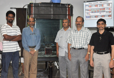
In recent years, in your work at JNCASR, you have been focussing more on cloud formation. You’ve assembled a cloud chamber which allows you to artificially generate clouds?
RN: First of all, the work really started at the Centre for Atmospheric and Oceanic Sciences (CAOS) at IISc. We are not actually generating clouds, we are generating cloud flows. I’ll make a distinction between the two. The reason for making the distinction between the two is that a cloud will have to have water vapour, water droplets, aerosols, radiation, etc, and the water vapour should be condensing and releasing heat.
What we are saying here is that cloud formation is primarily a complex fluid dynamical problem. The question is whether the simplest version of this otherwise complex fluid dynamical problem can be put together, where the flow behaviour has the same basic flow characteristics as that of a real cumulus cloud, that is, their shape, growth rate, entrainment characteristics, etc. Even if it can be done at least to a first rational approximation, then the other details can be progressively included.
Now it is not true, incidentally, that no one has yet attempted such models. J. Stewart Turner at Cambridge was a pioneer, but cloud shapes could not be reproduced. It seemed extraordinary to me that here is one problem where we don’t even understand the fundamentals of a phenomenon we see with our eyes everyday, and is furthermore at the heart of the monsoons and global climate change. However, there are now a small number of such groups.
There have also been mathematical models for clouds, but they make a large number of assumptions and differ widely from each other. It is a bit like the way engineers do turbulent flows. So it seemed to me once again that the problem really badly needed to be done, but had not attracted sufficient attention. That was the sort of thing I was looking for, so I started the project on clouds. And our first significant experiments were in the PhD thesis of G.S. Bhat.
About two years ago, there was a paper in Nature9 which spoke about the accuracy of short-term weather prediction. It argued that if you look at the forecast horizons of one-day and three-day forecasts, they have been getting consistently better. How is that possible when we don’t seem to have a handle on cloud formation?
RN: They said it is getting better. They didn’t say it was very good. [Laughs] They are getting better, that is true. They are getting better partly because cloud models are improving and getting more sophisticated, and computers have gotten more powerful and we have a lot more data from observations. I think we are quite close to being able to do what are known as Large Eddy Simulations (LES) for looking at these clouds. But there was also another Nature article more recently which appealed to physicists to save our planet by doing much more research on clouds!
But, even in those models, if you ask “Can you tell me the mechanics of what is happening inside the cloud?”, you will not be able to tell a great deal.
A Mathematical Model of Airworthiness: The Avro Story
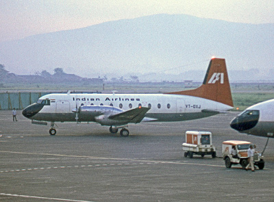
There are a couple of applied projects from your publication record which stood out for us. One project was an investigation that you carried out in the 1970s on this aircraft called the Avro 748, to check its airworthiness. This seems very different from all the theoretical investigations that you’ve carried out in fluid mechanics. How did it come about?
RN: Well, one fine day, 1 December 1970, to be precise, the Indian Airlines (IA) pilots flying the Avro 748 just walked off the aircraft and refused to fly it, saying that the aircraft was unsafe because the climb rate was below the prescribed British civil airworthiness regulations. So a lot of flights had to be cancelled.
That was the problem. What the government did was to appoint committees to investigate whether the aircraft was safe or not.
Was this the only aircraft in service at the time?
RN: Indian Airlines flew the 748 on its short-haul routes like Bombay–Pune and Bangalore–Chennai.
My interest in the problem was triggered by an interest in stochastic processes
Following the crash of a 748, the government appointed Satish Dhawan as a one-man committee to investigate the airworthiness of the aircraft. What Dhawan did was to set up an advisory committee with representatives from the industry, Air Force and DGCA [Directorate General of Civil Aviation], and also an Analysis Group consisting of scientists from the Institute [IISc], NAL [National Aerospace Laboratories] and HAL [Hindustan Aeronautics Limited].
It took us a while to figure out the rationale for the civil airworthiness regulations of that time. The British had the first major aviation regulations that specified a variety of technical performance parameters. I did a variety of studies, one of which was to find out if the Avro was actually unsafe, that is, to look at the number of accidents it had suffered. So I just got all the data on it from DGCA and from other countries. I found out that the accident rate of the Avro 748 was not very different from that of any other aircraft.
It wasn’t significantly more unsafe than other aircrafts?
RN: The record didn’t show that it was significantly more unsafe. So then I began to ask, “How are the British running this aircraft?” because they were allowing it to fly with a lower climb gradient than specified in their airworthiness regulations.
Even though it violated their own airworthiness criteria?
RN: Apparently so, and with good reason as it turned out. Anyway, we carried out a lot of tests on the aircraft, its engines and so on.
These were tests where the aircraft was actually flown?
RN: Including, but not limited to, ones where the aircraft actually flew on one engine. I still remember when the first such flight test was made. Dhawan was there, I was there, and some of the members of the advisory committee were there. The pilot was someone who was known and respected as one of the best at that time, Wing Commander Padmanabha Ashoka. Ashoka, after he retired from the Air Force, was the test pilot for HAL and thereafter worked at NAL for some years.
So the test pilot had to fly the aircraft in these tests where you take off, and at a certain point, he had to switch one engine off.
It was a twin-engine propellor aircraft?
RN: That’s right. And the problem was about the climb gradient when only one engine was on.
When the aircraft is moving on the ground, there is a decision speed. As soon as the aircraft exceeds that speed, the decision to take off is made and the pilot is not supposed to do anything but take off and climb, even if an engine fails.
Although Ashoka joked about it—he would say “If I disappear behind the trees, please go tell my wife!” [Laughs]—the flights went off without a hitch, and we finished in one day the flight tests that were supposed to be done over three days.
I had the responsibility to see that the technical work was done, that predictions were made for the climb rate, the data was analyzed by us, and so on. There was always this other question of why the British considered this plane airworthy. We had no experience with flight tests the way the British had. The British based it on their practical experience with the DC3 [the Dakota]. The regulations were made at a time, the 1930s, when the Dakota had become very popular.
We spent two years getting reliable data on how the performance of the aircraft and the engine and, in particular, how the climb gradient varied over time.
We could not repeat the studies that the British had made—we did not have the data. So I thought we could make a mathematical model which was what I called a stochastic corrective process. In this process, you have maintenance which improves the performance because otherwise, you will have a continuous deterioration of performance. What the data showed, for a parameter like climb gradient or engine power, was a time series of sudden jumps (after a maintenance check) and a slow deterioration between checks. All the variables involved were statistical in some sense. This suggested that the time series of performance is what may be called a stochastic corrective process (correction of deterioration by maintenance checks).
But acquiring accurate flight data was no routine task; in fact, getting thrust = mass \times acceleration was not a simple thing, as the thrust value was needed during flight. When this was finally achieved and announced by our friends from NAL and HAL at a meeting of the analysis group, the late Dr. Rustom Damania, the rare pilot with a PhD on the IISc faculty, joyfully said “Aha! Newton was right!”
So to cut a long story short, we made that stochastic process model into which we put all these things. We then did a Monte Carlo simulation of the stochastic process that defines the variation of aircraft performance that drops slowly but is recovered by short checks.
If you could visualize this stochastic process, is it one where some measure of the aircraft’s performance, like the climb rate, has a high probability that it declines over time?
RN: No, I wouldn’t say that. The correct way to put it would be that the stochastic process takes into account the deterioration. The deterioration is occurring, there is no doubt about it. However, when the engine is fresh from maintenance, it is actually giving you a thrust that’s more than what you need. And then, over time, that thrust comes down. In a good design, you make sure that it never goes below what you need for meeting airworthiness regulations and that depends on the maintenance process.
So, what our model did was that it took the deterioration data in India, factoring in our atmosphere, temperature, maintenance systems and so on. So it was very India-specific to begin with. And we had to make a large number of tests, and we then fed the real observed probability distribution of performance into the Monte Carlo code, which was written by Dr. N. Ramani, who was earlier my colleague at IISc.
We found that the probability of an accident was actually quite small, and we had to first of all convince our own team about the result. [Laughs] So, why was the probability of an accident so low? The answer was that the Avro 748 was powered by two Rolls Royce turbo-prop engines. The Dakota, on which the British had based their airworthiness regulations, had piston engines. The engine failure probabilities had dropped down drastically after the introduction of turbine engines, which are inherently safer because of fewer moving parts.
So, that is what was happening. There were few accidents of the 748 during climb because the failure rates of the engines were low. Thus, the 748 was safe to fly even though it didn’t clear the British airworthiness regulations. To test this view, I wrote to Sir Frederick Tymms, a respected leader who had by then retired from the British Civil Aviation Authority (CAA). He wrote to me agreeing with me, but pointed out that the British CAA has the freedom to interpret the code and accept certain concessions as long as they are convinced that the overall safety of the aircraft is not compromised. They hadn’t changed the code because there were other engines that were not yet so reliable.
To summarize, my interest in the problem was triggered by an interest in stochastic processes. After all, turbulence is a stochastic process. My experience with the Boltzmann equation had given me familiarity with Monte Carlo programmes. Thus, while the problem had nothing to do with fluid mechanics as such, the methods we had learnt in fluid mechanics were precisely the ones required for looking at airworthiness.
Anyway, Dhawan was satisfied, and the others were impressed. They couldn’t find anything to which they could object, so the report was sent. After the Dhawan committee’s report was submitted, we sent a paper to the Bulletin of the International Civil Aviation Organization,10 just to make sure that nobody would object outside after the problem was solved here. They accepted it, and in the paper, we gave a brief account of what we had done. I also wrote a more theoretical account of the stochastic corrective process.11
I could not publish the aircraft data we had to assess the value of the theory, but fortunately we came across extensive observational data on track-keeping errors of aircraft flying over the North Atlantic. The data was acquired for a project on collision avoidance. As deviations are seen on track-keeping, corrections are made; so this is another interesting example of a stochastic corrective process. Comparison of the theoretical distributions with observations showed excellent agreement.
Over these two interviews, we have talked about turbulence in various contexts. In that connection, there’s this quote by Richard Feynman: “If we watch the evolution of a star, there comes a point where we can deduce that it is going to start convection, and thereafter we can no longer deduce what should happen. A few million years later the star explodes, but we cannot figure out the reason.”
RN: [Laughs] I believe it.
As Feynman also said, turbulence is the last unsolved problem of classical physics
Could you summarize what makes this class of problems so difficult?
RN: It is simply that when the flow goes turbulent, we don’t understand it. Now, what Feynman was really saying was that as long as turbulence doesn’t come into the picture, we can handle the physics of the star, for example. After turbulence sets in, you are in the same situation as we are now on Earth. But once convection becomes turbulent, the fundamental problem of turbulence becomes a barrier. As Feynman also said, turbulence is the last unsolved problem of classical physics.
On that note, thank you very much for your time. We’ve had a lovely conversation with you. That’s all from us at Bhāvanā. Thank you.
RN: Thank you very much, it has been a pleasure to talk to you.
acknowledgement We thank Anupam Ghosh of ICTS for facilitating this interview.
Footnotes
- E. Mollo-Christensen and R. Narasimha. 1960. Sound Emission From Jets at High Subsonic Velocities. Journal of Fluid Mechanics. 8(1): 49–60. ↩
- R. Narasimha. 1960. Nearly Free Molecular Flow Through an Orifice. Physics of Fluids. 3: 476–477. ↩
- R. Narasimha. 1961. Orifice Flow at High Knudsen Numbers. Journal of Fluid Mechanics. 10(3): 371–384. ↩
- R. Narasimha. 1962. Collisionless Expansion of Gases into Vacuum. Journal of Fluid Mechanics. 12(2): 294–308. ↩
- R. Narasimha. 1961. Some Flow Problems in Rarefied Gas Dynamics. PhD thesis at Caltech. https://thesis.library.caltech.edu/4400/1/Narasimha_r_1961.pdf. ↩
- R. Narasimha. 1968. Asymptotic Solutions for the Distribution Function in Non-Equilibrium Flows. Part 1. The Weak Shock. Journal of Fluid Mechanics. 34(1): 1–24. ↩
- R. Narasimha and K.R. Sreenivasan. 1973. Relaminarization in Highly Accelerated Turbulent Boundary Layers. Journal of Fluid Mechanics. 61(3): 417–447. ↩
- R. Narasimha and K.R. Sreenivasan. 1979. Relaminarization of Fluid Flows. Advances in Applied Mechanics. 19: 221–309. ↩
- P. Bauer, A. Thorpe, and G. Brunet. 2015. The Quiet Revolution of Numerical Weather Prediction. Nature. 525: 47–55. ↩
- R. Narasimha. 1974. A Statistical Approach to Airworthiness and Flight Safety. Proceedings of First Seminar on Flight Evaluation: 80–94. ↩
- R. Narasimha. 1975. Performance Reliability of High Maintenance Systems. Journal of the Franklin Institute. 303(1): 15–28. ↩