The Tangled History of the String Equation

Think of your favourite stringed instrument. Each metallic wire on it likely has a different thickness or diameter, and is stretched to provide a precise amount of tension in it. These are the factors that determine which note can be played with it. Left untouched, such an instrument is a mere bundle of stretched strings.

Until you pluck one of them. The pluck further stretches the already taut string. The moment you let go, two kinds of waves start to travel through it. Longitudinal waves move along the string, while transverse waves move in the other two spatial directions that are at right angles to the string. The final note you will hear is not born from the vibration of the string itself, but through the vibration of the rest of the instrument induced by the waves coursing through the string. Perhaps an artiste need not be concerned with the interplay of Newton’s laws in a stringed instrument to produce a melody. But to some, the science of tracing the rapid motion of this string is as exciting as the final note itself.

That was indeed the case with Gustav Kirchhoff, George Carrier, and Roddam Narasimha. All three of them worked out equations that can be used to predict the behaviour of a vibrating string. Despite the popularity of each of their models of string behaviour, and the differing assumptions they made en route to deriving these models, the scientific literature has been inconsistent in ascribing authorship of each of these models. After exploring the assumptions and motivations that gave rise to each of the equations, we aim to convince the reader that the names commonly associated with equation \eqref{kirchh} in literature do not adequately reflect its history.

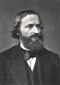
Gustav Kirchhoff (1824–1887), a German physicist, derived an equation for the vibration of strings from an earlier equation he had derived to understand the vibration of thin beams [1]. We will not follow the original derivation of Kirchhoff’s equation, but will explore the intuition behind the terms that appear in it. One possible derivation of Kirchhoff’s equation, parts of which we motivate below, can be seen in [2]. This derivation sets the tone to explore the contributions of Kirchhoff, Carrier and Narasimha towards our understanding of string vibrations.

Consider a string of length l and cross-sectional area A that is fixed at both ends. The string has a tension T_0 along its length while it is at rest. When the string is stretched as shown in Figure 1, an infinitesimal element of length ds on the resting string increases in length to ds' after the string is stretched. We will consider vibrations of the string only in a plane, which means there is only one transverse direction. The components of the length ds' along the x and y directions are (1+u_x)\,ds and w_x\,ds, respectively; u and w are longitudinal and transverse displacements, which are tangential and perpendicular to the element ds, respectively, and u_x and w_x represent the partial derivatives in the x-direction of motion.

The changed length of ds upon stretching is ds' = \epsilon \, ds = (\sqrt{(1+u_x)^2 + w_x^2}-1)ds. The quantity \epsilon is derived from what are called strain-displacement relations, which appear in the theory of elastic behaviour of materials. In the case of the strings we consider, the relations used in the derivation are valid when the string can deform only along its length while leaving its cross-section unchanged.

Aside from changing the length of the string, stretching also changes the tension within the string. When the string is at rest, the net tension on ds is zero. When the string is stretched and released, the net tension on ds' is non-zero, which causes its acceleration. If the longitudinal and transverse components of the net tension on ds' are T_u and T_w, Newton’s second law yields two equations

where \rho is the density of the string; u_{tt} and w_{tt} are second order partial derivatives of u and w with respect to t that represent the acceleration of the element in those directions, respectively. If \sigma is the stress in the string, which is the force per unit area that deforms the string, then the net tension T_1' - T_2' on ds' is T_0 + \sigma A. From the figure, it can be seen that the tension components T_u and T_w are

To complete the equations, a relation is needed between \sigma and \epsilon. If we assume that the material in the string follows Hooke’s law, then \sigma = E\epsilon, where E is the elastic modulus of the material. E is a measure of the force required per unit area of the string to deform it along its length. E tends to be large for metals, but is relatively smaller for materials like rubber or nylon. Substituting \sigma = E\epsilon = E\sqrt{(1+u_x)^2+w_x^2-1}, along with equations \eqref{tension1} and \eqref{tension2} into equation \eqref{newtonslaw}, gives the exact equations of motion for a string that satisfies Hooke’s law:

The first approximation needed to derive Kirchhoff’s equation from equations \eqref{newtonslawfull1} and \eqref{newtonslawfull2} is to approximate the strain \epsilon = \sqrt{(1+u_x)^2+w_x^2}-1. A common approximation is setting \epsilon \approx u_x + w_x^2/2, which is based on the assumption that both longitudinal and transverse vibration amplitudes are small. This simplifies the above equations to

The important point to note is that the first equation above, which describes longitudinal motion, contains the term w_x, which is a component of the transverse motion of the string. Similarly, the transverse motion described in the second equation depends on the longitudinal motion of the string. Thus, both transverse and longitudinal motions of the string are coupled to each other.

The second approximation made in equation \eqref{kirchhoff1a} to derive Kirchhoff’s equation is to assume the longitudinal motion of the string to be small enough to allow us to set u = 0. This eliminates the equation \eqref{kirchhoff1a} altogether and sets u_x = 0 in equation \eqref{kirchhoff1b}. Finally, if the tension A\sigma = EAw_x^2/2 is assumed to be constant along the string, \partial (A\sigma w_x)/\partial x can be replaced by its average value along the string, which is

Combining all the constants together, we obtain Kirchhoff’s equation for the transverse displacement of a string of length l

Kirchhoff’s derivation of equation \eqref{kirchh} differs from the one presented here. He originally derived an equation to model the planar vibrations of a thin beam, and considered the string to be a special case of a thin beam, one of whose spatial dimensions tends to zero. However, the assumptions imposed in our sketch of the derivation of Kirchhoff’s equation are the same as the assumptions imposed by Kirchhoff, namely, (a) the longitudinal motion of the string is neglected, (b) the amplitude of the transverse vibration is small, and (c) the additional tension across the string, at a given instant of time, is the same along the string.

Kirchhoff’s equation has been studied through numerical and analytical methods, with the conditions for the existence of solutions to \eqref{kirchh} being first studied in 1940. Despite its popularity, there has been much confusion regarding its origins. Starting from the 1970s, \eqref{kirchh} was referred to as the Carrier–Narasimha equation (see [3]). However, in the 1990s, it was realized that \eqref{kirchh} was actually derived by Kirchhoff [4]. While some now refer to equation \eqref{kirchh} as the Kirchhoff string equation (notably, [2] and [5], amongst others), some also refer to it as the Kirchhoff–Carrier equation [6].

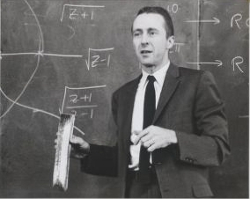
The equation that was derived by George Carrier (1918–2002), an American mathematician, in 1945 [7] is of the form

Carrier’s equation does not contain a derivative in the integral that represents the tension in the string, while Kirchhoff’s equation does. This difference arises because Carrier’s derivation does not impose the assumption that the amplitude of transverse vibration is small. In fact, in 1960, Donald Oplinger, who worked at the Mechanical Research Laboratory of DuPont, showed that it is possible to derive equation \eqref{kirchh} from equation \eqref{carr} [8] if the amplitude of transverse vibration is small, although he does not refer to equation \eqref{kirchh} as Kirchhoff’s equation. While Carrier didn’t impose this assumption on transverse vibrations, he still neglects the longitudinal displacement of the string. As it turns out, neglecting the longitudinal motion of the string leads to unexpected results when comparing Kirchhoff’s or Carrier’s equations to experiments built to study the vibrations of a stretched string.

Oplinger also performed experiments that studied the transverse vibrations of a stretched string. A picture of the apparatus he used is shown in Figure 2. Oplinger was interested in studying the vibrations of a string when one end of it is subject to a periodically varying external force. He stretched a wire made of nylon (which was, incidentally, invented at DuPont), one end of which was attached to strain gauge that helped measure the tension of the string. The other end was attached to a device that applied a periodically varying force to the string. The amplitude of the resulting motion was recorded with a measuring scale parallel to the plane of vibration of the string. Oplinger could vary the magnitude and frequency of this external driving force. When a driving force is applied to the string, the equations of motion of the string need to be modified to account for this force. This is done by adding the term F_0\cos(\omega_0) to the right hand side of Kirchhoff’s and Carrier’s equations, where \omega_0 is the angular frequency of the driving force. In Oplinger’s coordinate system, the string vibrates in the xy-plane that is parallel to the ground, while the components of the driving force are also only in the xy-plane.

For a string subject to a driving force, changes in \omega_0 lead to changes in the amplitude of transverse vibration of the string. There are certain values of \omega_0 at which the amplitude becomes very large. This phenomenon is called resonance. In a musical instrument like a guitar or veena, the vibration of the string is the driving force that excites the rest of the instrument through resonance. The resonant vibration of the entire instrument has sufficient energy to give rise to a musical note. Another often cited example of resonance is the swaying of a bridge when soldiers march across it in step with each other. In situations like the oscillations of a bridge, an experiment to measure its resonant frequency might actually damage the system being studied. In such a case, being able to calculate resonant frequencies is of critical importance.

Resonant frequencies for strings are tricky to calculate. By measuring the tension and amplitude of a nylon wire at different driving force frequencies, Oplinger attempted to derive a better model of string vibrations that would match measurements of resonant frequencies, and also understand why theoretically derived resonant frequencies deviated from measurement. Oplinger measured the amplitude of string vibrations at different driving force frequencies, and found that Kirchhoff’s equation could be used to calculate fairly accurate resonant frequencies, but only within a particular range of driving frequencies. Outside of this range, he found that the string behaved rather unexpectedly near certain resonant frequencies predicted by Kirchhoff’s equation. At these frequencies, though the driving force experienced by the string had no z-component, the string oscillated in the z-direction!

In 1948, Henry Harrison, an acoustics researcher, wrote in a letter to the editor of The Journal of the Acoustical Society of America that “It is not trivial to drive a bounded string so that it will vibrate in a plane. This fact, which is well known to laboratory instructors in elementary physics courses, was demonstrated again in an experiment carried out by J.K. Hunton in the Research Laboratory of Electronics, M.I.T.” [9]. Oplinger was aware of this prior observation. In fact, the reason he passed the nylon wire through a slit was to try and eliminate the motion of the wire in the z-direction. He did not pursue a theoretical explanation for this behaviour.

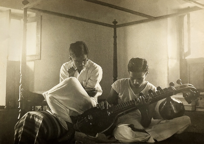
B.S. Ramakrishna (1920–2011), a professor at the Department of Electrical Communication Engineering at the Indian Institute of Science, Bangalore, noted the out-of-plane behaviour observed by Oplinger, and set out to understand its occurrence. Along with his student, G.S. Srinivasa Murthy, Ramakrishna published a detailed experimental and theoretical study of the out-of-plane vibration of strings in 1964 [10], where they showed that out-of-plane motion of a string near a resonant frequency was actually the norm rather than the exception. His experiments also showed that the resonant frequencies at which the in-plane transverse vibrations became large were different depending on whether the string also vibrated out of the plane.

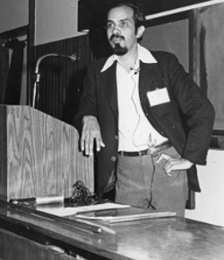
When Roddam Narasimha published his model of a vibrating string in the Journal of Sound and Vibration in 1968, he acknowledged this work, writing that “This paper owes its inspiration to the work of Professor B.S. Ramakrishna and his students.” [11]. Narasimha derived the following equation for the transverse displacement of a string under the influence of a driving force

R is a constant that represents the magnitude of damping in the string. Damping is what causes a vibrating string to eventually stop vibrating, in the absence of a driving force. \mathbf{w}(x,t)=(y(x,t),z(x,t)) represents the two transverse displacements of the string. In the integral, \mathbf{w}_x^2 = y_x^2+z_x^2, and \mathbf{f}(x,t) represents the driving force applied on the string in a plane that is normal to the x-axis. Note that neither Kirchhoff’s nor Carrier’s equations contain both transverse components.

In his derivation of the string equation, Narasimha argued that string vibrations where the longitudinal displacement u is zero, but w is non-zero, are possible only in very special instances. While Carrier’s derivation assumes the tension along the string at a given instant of time to be fixed, Narasimha does not impose this assumption. His derivation is general enough to not require the assumption of small longitudinal displacements to be imposed, although he does impose it to derive the equation in the form shown in equation \eqref{RN}.

Recall that in equations \eqref{kirchhoff1a} and \eqref{kirchhoff1b}, the transverse and longitudinal motions are generally coupled to each other. Setting the longitudinal displacement to zero in those equations uncouples the transverse component from the longitudinal one. While Narasimha recapitulates this feature of string vibrations, he goes on to show that the two transverse vibrations in his equation are also coupled with each other. Thus, under certain mathematical conditions, which are derived by him, in-plane transverse vibrations can lead to out-of-plane transverse vibrations when a vibrating string is driven by an external force.

The only assumption that Narasimha imposes at the beginning of his derivation is that deformations of the string follow Hooke’s law. With the exception of this assumption, Narasimha is able to do away with the assumptions made in Carrier’s and Kirchhoff’s equations, and shows the mathematical conditions under which they are reasonable approximations of string motion. His equations are also able to qualitatively match the different resonant frequencies measured when a string vibrates out of plane, as seen in Murthy and Ramakrishna’s experiments.

Narasimha’s work seems to have revived mathematical studies of equations with the same form as Kirchhoff’s equation, after J.L. Lions formulated Narasimha’s equation in an abstract framework, and proved the existence and uniqueness of its solution [12]. An interesting testimony to the mathematical rigour of Narasimha’s derivation comes from the response of Clifford Truesdell to Narasimha’s paper. Truesdell, a mathematician, historian and philosopher, was known for his efforts to put the study of mechanics on firm mathematical foundations. Jean-Pierre Meyer, a mathematician and a colleague of Truesdell, noted that Truesdell was infamous for being vocally critical of other faculty members [14]. While reviewing a certain other paper, Truesdell once commented [15] that

This paper… gives wrong solutions to trivial problems. The basic error, however, is not new…

However, as for Narasimha’s derivation, Truesdell’s only comment was to point out an incorrect use of nomenclature where Narasimha interchanged the terms “Eulerian” and “Lagrangian” while referring to the variables used in his equation. For more details on Narasimha’s derivation of the string equation, and other equations proposed to model string behaviour, see [13].

Considering the differences between the derivations of the three equations, the prevailing confusion around them is surprising. Amongst the three equations, Kirchhoff’s equation was the first chronologically. However, both Narasimha and Carrier were unaware of Kirchhoff’s derivation, and derived their respective equations with different physical assumptions. Each of the existing names used to refer to equation \eqref{kirchh}—Kirchhoff–Carrier or Carrier–Narasimha—leave unacknowledged a different route that has been independently explored to derive it. Oplinger also derived equation \eqref{kirchh} from Carrier’s equation, seemingly with no reference to Kirchhoff’s work. With many claimants to it, assigning a name to equation \eqref{kirchh} is thus a difficult proposition.

acknowledgement The authors would like to thank Vishaka Datta for his work on the exposition of the string equation and the historical narrative. In particular, we are grateful for his careful research and sensitive editing of our original draft, and for creating Figure 1.

References

• [1] G. Kirchhoff. Vorlesungen ūber Mathematische Physik: Mechanik. 1876. Druck und Verlag von B.G. Teubner, Leipzig
• [2] L.Q. Chen, H. Ding. Two Nonlinear Models of a Transversely Vibrating String. Arch. Appl. Math. 2008. 78: 321–328
• [3] A. Arosio. Global (in time) Solution of the Approximate Nonlinear String Equation of G.F. Carrier and R. Narasimha. Comment. Math. Univ. Carolin. 1985. 26: 166–172
• [4] S. Spagnolo. The Cauchy Problem for the Kirchhoff Equations. Proceedings of the Second International Conference on Partial Differential Equations (Italian) (Milan, 1992). Rend. Sem. Fis. Mat. Milano. 1992. 62: 17–51
• [5] J. Peradze. A Numerical Algorithm for the Nonlinear Kirchhoff String Equation. Numer. Math. 2005. 102: 311–342
• [6] S. Bilbao. Modal-Type Synthesis Techniques for Nonlinear Strings with an Energy Conservation Property. Proc. of the 7th Int. Conf. on Digital Audio Effects (DAFx’04), Rome, Italy. 2004
• [7] G.F. Carrier. On the Nonlinear Vibration Problem of the Elastic String. Q. J. Appl. Math. 1945. 3: 157–165
• [8] D.W. Oplinger. Frequency Response of a Nonlinear Stretched String. J. Acoust. Soc. Am. 1960. 32: 1529–1538. DOI: 10.1121/1.1907948
• [9] H. Harrison. Plane and Circular Motion of a String. J. Acoust. Soc. Am. 1948. 20: 874–875
• [10] G.S. Srinivasa Murthy and B.S. Ramakrishna. Nonlinear Character of Resonance in Stretched Strings. J. Acoust. Soc. Am. 1965. 38: 461–471
• [11] R. Narasimha. Nonlinear Vibration of an Elastic String. J. Sound Vib. 1968. 8: 134–155
• [12] J.L. Lions. On Some Questions in Boundary Value Problems of Mathematical Physics. Published in: G.M. de La Penha, L.A. Medeiros (Eds.) Contemporary Developments in Continuum Mechanics and Partial Differential Equations, North-Holland, Amsterdam. 1978. 30: 284–346
• [13] A.S. Vasudeva Murthy. On the String Equation of Narasimha. Connected at Infinity II: A Selection of Mathematics by Indians. 2013. Hindustan Book Agency
• [14] G. Brown. Renaissance (math)man, The Johns Hopkins Magazine. June 2009. 61(3)
• [15] C. Truesdell. MR0039515 (12, 561a)