1 Introduction
The deep regard that P.C. Mahalanobis had for the mathematical and scientific intellect of ancient India is expressed in the very name Sankhyā that he chose for the journal on statistics that he founded in 1933. In the inaugural editorial of Sankhyā [1], as also in his celebrated article “Why Statistics?” [2], Mahalanobis highlights some of the ancient Indian ideas on administrative statistics, and remarks that the Arthaśāstra of Kauṭilya “contains a detailed description for the conduct of agricultural, population, and economic censuses in villages as well as in cities and towns on a scale which is rare in any country even at the present time. The detailed description of contemporary industrial and commercial practice points to a highly developed statistical system.” ([2], p. 196)
As a tribute to P.C. Mahalanobis on his 125th birth anniversary (he was born on 29 June 1893), we mention a few of the several formulations and applications of the Arithmetic Mean that occur in the works of ancient Indian mathematicians.
We first make a few introductory remarks on the concept of the Arithmetic Mean and its history.
1.1 Arithmetic Mean in Mathematics and Statistics
In mathematics, the Arithmetic Mean \overline{x} of n numbers x_1, x_2, \ldots, x_n is formally defined to be the number
\[\begin{equation}\label{eq0}
\overline{x}=\frac{x_1+x_2+\cdots+x_n}{n}.
\end{equation}\]
It is an exact mathematical concept. But it is widely applied in the study of approximations. For, the concept appears in the experimental sciences in its following avatar: the Arithmetic Mean of measurements in a recorded data is the sum of all the measurements divided by the number of measurements. And physical measurement is something intrinsically approximate.
There is another way of looking at the dual role of the Arithmetic Mean as a “pure” cum “applied” concept. Practical experience shows that numbers in statistical data usually tend to cluster around some central value. Any estimate (or measure) of this “central tendency” (also called “average”) seeks to identify that typical or central value of the distribution which would, in some sense, be its best representative. The Arithmetic Mean, Median and Mode are three standard measures of central tendency used in statistics. Thus, the precise arithmetic (rather, algebraic) formula \(\eqref{eq0}\) is viewed in statistics as an estimate of the central tendency of a distribution.
When the n quantities x_1, x_2, \ldots, x_n are assigned weights w_1, w_2, \ldots, w_n respectively, then the more general concept “weighted arithmetic mean” \overline{x} is defined as
\[\begin{equation}\label{eqw}
\overline{x}= \frac{w_1x_1+\cdots+w_nx_n}{w_1+\cdots+w_n}.
\end{equation}\]
1.2 The Popularity and Importance of the Arithmetic Mean
The Arithmetic Mean (A.M. in short) is frequently used not only in statistics and mathematics, but also in experimental science, economics, sociology, and other diverse academic disciplines. Geometrically, the arithmetic mean [equation \(\eqref{eq0}\)] captures the concept of the “centre” of a configuration — the coordinates of the “centroid” of a triangle (or any other figure bounded by line segments) is the Arithmetic Mean of the coordinates of the vertices. In physics, the weighted A.M. [equation \(\eqref{eqw}\)] appears in the form of the “centre of mass”. For a set of n points with coordinates \mathbf{r_i} and masses m_i, the coordinates of the centre of mass is the weighted A.M. (m_1\mathbf{r_1}+\cdots+m_n\mathbf{r_n})/(m_1+\cdots +m_n).
The definition of the Arithmetic Mean [equation \(\eqref{eq0}\)] is elegant, easy to understand, and it is straightforward to write a computer programme for computing the Arithmetic Mean. It is therefore not surprising that the Arithmetic Mean has been the most commonly used measure of central tendency and the word average has practically become a synonym for the Arithmetic Mean. Apart from being a measure of central tendency, the A.M. is also a useful parameter for insights into other features of a given data like the variance or the standard deviation which measure the tendency of dispersion in the data. Some of the deeper conceptual aspects of the Arithmetic Mean are mentioned in section 2.5.
In a special lecture at the Indian Statistical Institute, Kolkata, on the First World Statistics Day (20.10.2010), S.M. Stigler1 singled out the Arithmetic Mean as the first of the “Five Ideas that Changed Statistics and Continue to Change the Way We Think About the World”. The basic idea at the heart of the Arithmetic Mean is to combine observations—to replace several numbers by a single number. Thinkers on statistics like Stigler [24] have pointed out that this idea is counterintuitive: for it seeks, paradoxically, to gain information about the data by discarding information, namely, the individuality of the observations. Besides, in the words of Stigler ([24], p. 14):
In ancient and even modern times, too much familiarity with the circumstances of each observation could undermine intentions to combine them. The strong temptation is, and has always been, to select one observation thought to be the best, rather than to corrupt it by averaging with others of suspected lesser value.
Thus, although the Arithmetic Mean (like the decimal system) now seems a natural concept to us who have grown up with it, its introduction must have needed a conceptual subtlety. The idea of A.M. as a statistical estimate appears in scientific treatises of Europe quite late.
1.3 Antiquity of the Arithmetic Mean
Several scholars on history of statistics have been asserting that it is only from the 17th century ce that one comes across the use of the Arithmetic Mean as a representative value for any data comprising more than two observed values. They see in a work dated 1635 of the English astronomer Henry Gellibrand the earliest unambiguous use of the Arithmetic Mean in a statistical sense. In his presidential address at the American Statistical Association in 1971, Churchill Eisenhart remarks ([8], p. 14):
… I fully expected that I would find some good examples of mean taking in ancient astronomy; and, perhaps, also in ancient physics. I have not found any. And I now believe that no such examples will be found in ancient science.
Eisenhart observes that ancient scientists did not have any precise method for choosing a best estimate on the basis of several observations—they relied on adroitly chosen observations. But, as in the case of numerous other scientific concepts, such an account of history completely overlooks the clear and precise use of the Arithmetic Mean in the treatises of ancient Indian mathematicians like Brahmagupta (628 ce), Śrīdharācārya (c. 750 ce), Mahāvīrācārya (850 ce), Pṛthūdakasvāmī (864 ce), Bhāskarācārya (1150 ce) and others. In fact, as we shall illustrate in sections 3 and 4, these Indian mathematicians define and apply the more general and sophisticated concept of weighted Arithmetic Mean [equation \(\eqref{eqw}\)]. An intuitive awareness of the law of large numbers for A.M. also comes out in a commentary by the mathematician Gaṇeṣa (1545 ce)—see section 3.6.
In section 3, we shall quote statements on A.M. from chapters in Indian arithmetic called khāta-vyavahāra (mathematical processes pertaining to excavations). These chapters describe how to compute the (average) depth, width or length of an irregular-shaped pool of water and thereby estimate its volume. It is in these chapters that the Arithmetic Mean is defined and used in a statistical sense, i.e., as the best representative value for a set of observations. Brahmagupta is one of the earliest Indian mathematicians in whose text the concept of Arithmetic Mean (in fact, weighted A.M.) occurs explicitly in this statistical sense. He uses it to represent the depth of a ditch, when the depth is different in different portions of the ditch. But perhaps the numerous novel ideas in the work of a colossus like Brahmagupta have overshadowed this occurrence of the Arithmetic Mean in his work.2 Very recently, Brahmagupta’s work has been acknowledged by Stigler in [24] (p. 30).
As mentioned earlier, the Arithmetic Mean “combines” several numbers into a single number. Ancient Indian mathematics, especially the mathematics of Brahmagupta, appears to be replete with various ideas of “combination”. In the inaugural issue of Bhāvanā, we had seen that Brahmagupta had introduced a principle of composition which combines two solutions of a certain quadratic equation in three variables to produce another solution of the equation, a principle with momentous consequences in mathematics [6]. In fact, the name of this publication is inspired by the term bhāvanā used in Indian mathematics for Brahmagupta’s law of composition. Since “(finding by) combination” is one of the meanings of the Sanskrit word bhāvanā ([6], p. 14), one can view the Arithmetic Mean too as the outcome of a bhāvanā!
In section 4, we shall quote statements on A.M. from chapters in Indian arithmetic called miśraka-vyavahāra (computations pertaining to mixtures) which address the problem of computing the proportion of pure gold in an alloy formed by blending of several pieces of gold of different weights and purities. Here, weighted Arithmetic Mean appears as an exact mathematical concept rather than as a representative or an estimate in a statistical sense. However, even for scholars interested primarily in the history of the statistical Arithmetic Mean, the passages on miśraka-vyavahāra may give a perspective regarding the mathematical environment which facilitated the emergence of this statistical idea. Apart from problems on combining gold pieces, there are other contexts, like problems of combining different investments (with simple interest) into an equivalent single investment, which have also led to calculations of weighted Arithmetic Mean. They will not be discussed in the present article. In their planetary models, ancient Indian astronomers routinely discuss the “mean motion” of a planet which too will not be discussed in this article.
In Indian treatises on arithmetic, the topic miśraka-vyavahāra is discussed much before the topic khāta-vyavahāra. We have however highlighted the verses from khāta-vyavahāra first (i.e., in section 3) because of their immediate relevance for the history of the Arithmetic Mean in its statistical sense.
1.4 Ancient Indian Terms for the Arithmetic Mean
The formula for weighted arithmetic mean [equation \(\eqref{eqw}\)] appears in the earliest available ancient Indian texts using A.M. and there is no distinction in Sanskrit terminology between the arithmetic mean [equation \(\eqref{eq0}\)] and the weighted arithmetic mean [equation \(\eqref{eqw}\)].
The Sanskrit word sama (whose meanings include: “equal”, “equable”, “same”, as well as “common”, “mean”) is the technical term employed by ancient Indian mathematicians for the (weighted) Arithmetic Mean. The word rajju denotes “rope”, “string”, “cord” (i.e., instruments for measurements of lengths), a line segment (i.e., that which is to be measured), as well as “the measure of a line segment”. The term samarajju (mean measure of a line segment) is used by Brahmagupta (628 ce) and Pṛthūdakasvāmī (c. 864 ce) for the (weighted) Arithmetic Mean.
Other forms in which the (weighted) Arithmetic Mean occurs in Indian texts include ([10], p. 136): samīkaraṇa (levelling, equalizing) by Mahāvīrācārya (850 ce), sāmya (equality, impartiality, equability towards) by Śrīpati (1039 ce) and samamiti (mean measure) by Bhāskarācārya (1150 ce) and Gaṇeṣa (1545 ce). The terminology shows that the Arithmetic Mean was perceived by ancient Indian scholars as the “common” or “equalizing” value which would be the appropriate representative measure for various observed measurements.
2 Arithmetic Mean in Europe
2.1 Arithmetic Mean of Two Numbers in Ancient Greece
Ancient Greeks like Pythagoras (c. 500 BCE) defined the Arithmetic Mean of two numbers x_1 and x_2 with x_1 < x_2 to be the “middle number” x equidistant from x_1 and x_2, i.e., a number x satisfying x_2-x=x-x_1. In fact, the term mean is etymologically related to the Old French meien which means “middle” or “centre” whose descendants include the Middle French moien and its variant meen and the Middle English mene.
Now, if x_2-x=x-x_1 then x=(x_1+x_2)/2, and vice versa. Thus, for two numbers x_1, x_2, the ancient Greek definition for the A.M. of two numbers is clearly equivalent to the modern definition of A.M.
However, note that the Pythagorean definition envisages the Arithmetic Mean as a geometrical concept (the midpoint of a line segment) and not as the statistical concept of “average” or as “the best representative” among (or as a substitute for) several numbers. It was used in the context of music and pure mathematics, and not in analysis of data.
In their account on the history of the Arithmetic Mean and the Median, Bakker and Gravemeijer write ([3], p. 154):
Not until the sixteenth century was it recognized that the arithmetic mean could be generalized to more than two cases: a=(x_1+x_2+\cdots+x_n)/n.
It is another matter that the above statement becomes incorrect if we take into account ancient Indian mathematics, but the observation is indeed valid if we restrict to what is currently known about the history of science in Europe. This history suggests that the geometric conceptualization by the Greeks of the A.M. as the “middle of two numbers” has not been conducive for generalization to n numbers, although it is mathematically equivalent to the modern computational formulation (x_1+x_2)/2. We shall continue this discussion in section 5.2.
2.2 The Use of the Mid-Range
There are instances of a certain generalization of the Pythagorean A.M. for two numbers which could be a possible precursor to the modern A.M. for n numbers (for any n). This is the notion of what is now called the “mid-range” of n numbers: the Arithmetic Mean of the largest and the smallest of the n numbers. The idea of the mid-range appears in the work of the Greek historian Thucydides of the 5th century BCE ([3], p. 152) and the Arab writer al-Biruni of the 11th century ce ([8], pp. 31–36).
2.3 Probable Use of Arithmetic Mean by Tycho Brahe
R.L. Plackett suggests ([13], p. 122) that the “technique of repeating and combining observations made on the same quantity appears to have been introduced into scientific method by Tycho Brahe towards the end of the sixteenth century”. It is quite likely that Tycho Brahe (1546–1601) uses the Arithmetic Mean but, as pointed out by Eisenhart ([8], p. 40), he does not define or even mention the A.M. explicitly. Moreover, as he records the summary (i.e., the average) of observations as a rounded value (e.g., he would write 26^{\circ} 0^{\prime} 30^{\prime \prime} rather than 26^{\circ} 0^{\prime} 27^{\prime \prime} or 26^{\circ} 0^{\prime} 29^{\prime \prime} —see [13], p. 123), there is an ambiguity regarding which “average” (A.M., mid-range, median, mode, any other) is actually applied by Tycho Brahe.
2.4 Arithmetic Mean in Geomagnetic Studies
During the 15th century, Europe entered the “Age of Exploration”, an era marked by a zest for expeditions and a search for new sea-routes. This period witnessed new scientific investigations related to navigation. One such prominent theme of scientific research was magnetic declination (earlier called “variation of the compass”)—the angle between the magnetic north and the true north. Towards the end of the 15th century, it was found that there are marked differences in the observed measurements of the magnetic declination in different parts of the world. The measurement of magnetic declination “was pursued with diligence throughout the 16th and the early part of the 17th centuries” ([8], p. 56).
Eisenhart [8] has traced the evolution of what he calls “mean taking” in writings on magnetic declination. In the late 16th century, a recommendation to use the mid-range can be seen ([8], pp. 48–50) in discussions on the magnetic declination in the works of Thomas Harriot (1595) and Edward Wright (1599).
In 1580, William Borough (1536–1599) records nine readings of the magnetic declination at Limehouse in London’s East End, using morning and afternoon shadows corresponding to Sun altitudes 17, 18, …, 24 and 25^{\circ} ([8], p. 62). The nine declination values are 11^{\circ} t^{\prime} E, the nine values of t being: 17 \frac{1}{2}, 11 \frac{1}{2}, 30, 22 \frac{1}{2}, 22 \frac{1}{2}, 15, 20, 17, 14. By “… conferring them altogether”, Borough estimates the true declination to be about 11 \frac{1}{4} or 11 \frac{1}{3} degrees (i.e., 11^{\circ} 15^{\prime} or 11^{\circ} 20^{\prime}). Note that the exact Arithmetic Mean of the nine observations is 11^{\circ} {18 \frac{8}{9}}^{\prime}.
The unusual expression “conferring them altogether” suggests that Borough might have computed the Arithmetic Mean (a term which will be explicitly mentioned by a later astronomer who analyzed his findings) and the mixed fractions 11 \frac{1}{4} and 11 \frac{1}{3} could be convenient “coarsely rounded values of the arithmetic mean” ([8], p. 61). Eisenhart mentions a few other possible instances of “mean-taking” in the 16th century and concludes ([8], p. 53):
These examples are, of course, conjectural, but I have a feeling that some clear-cut examples of “mean-taking” in navigational settings may well be lying “buried” in the logs and chronicles of one or another of the 16th century voyages of exploration, awaiting discovery by alert attuned eyes.
In the 17th century, the astronomer Henry Gellibrand (1597–1636) discovers that, even at a fixed place, the magnetic declination varies with time. The term Arithmeticall meane occurs explicitly in his work (1635). From observed declinations 11^{\circ} and 11^{\circ} 32^{\prime} 28^{\prime \prime}, he estimates the declination to be about 11^{\circ} 16^{\prime}, a rounded value of the exact A.M. 11^{\circ} 16^{\prime} 14^{\prime \prime}. From observed declinations 4^{\circ} 6^{\prime}, 4^{\circ} 10^{\prime}, 4^{\circ} 1^{\prime}, 4^{\circ} 3^{\prime}, 3^{\circ} 55^{\prime}, 4^{\circ} 7^{\prime}, 4^{\circ} 10^{\prime}, 4^{\circ} 12^{\prime}, 4^{\circ} 4^{\prime}, 4^{\circ} 0^{\prime} and 4^{\circ} 5^{\prime}, he assigns the declination to be around 4^{\circ} 4^{\prime}, which is again a rounding down of the exact A.M. 4^{\circ} {4 \frac{9}{11}}^{\prime}. Though he does not define the Arithmetic Mean and, in each of the above cases, the mid-range too matches his assigned estimate, Eisenhart feels that the term Arithmeticall meane makes it highly probable that Gellibrand is indeed referring to the A.M. in its current sense ([8], pp. 64–66).
A more clear-cut use of the A.M. as the best approximation for the true value can be seen ([8], pp. 68–69) in an extract of a letter published in the Philosophical Transactions (1668) informing that Captain Samuel Sturmy made 5 declination measurements 1^{\circ} 22^{\prime}, 1^{\circ} 36^{\prime}, 1^{\circ} 34^{\prime}, 1^{\circ} 24^{\prime}, and 1^{\circ} 23^{\prime}; and took the “mean” to conclude the declination to be 1^{\circ} 27^{\prime}. For this data, the exact A.M. is 1^{\circ} {27 \frac{4}{5}}^{\prime}, the Median 1^{\circ} 24^{\prime} and the mid-range 1^{\circ} 29^{\prime}; so Sturmy’s “mean” undoubtedly refers to our Arithmetic Mean!
By the middle of the eighteenth century, the (simple) arithmetic mean was in frequent use in astronomy and navigation, for a small set of measurements made under essentially the same conditions and usually by the same observer [13]. However, the use of statistical weighted A.M. to combine measurements was rare in Europe before 1750. A work of Roger Cotes (published posthumously in 1722) contains a rule ([23], p. 16) which appears to recommend the use of a weighted arithmetic mean.3
2.5 Sophisticated Insights on the Arithmetic Mean
The work of P. Laplace (1749–1827), A.M. Legendre (1752–1833) and C.F. Gauss (1777–1855) provides a firm theoretical foundation for the Arithmetic Mean. The concept of the Arithmetic Mean is central to the method of least squares in the theory of errors introduced by Legendre (1805) and Gauss (1809).4 To see this, consider n given numbers x_1, \ldots, x_n and an arbitrary number x, and note that each difference x_i-x is the “error” if x_i is substituted by x. It can be shown mathematically that as x varies over real numbers, the value of x for which the sum of squares of the “errors”
\[
(x_1-x)^2 + \cdots + (x_n-x)^2
\]
is the minimum, is exactly the Arithmetic Mean \overline{x} of x_1, \ldots, x_n. This precise mathematical result showing that the A.M. minimises the error in substituting all the numbers x_1, \ldots, x_n by a common value x gives the theoretical justification for considering the A.M. as the “best representative” for the given numbers. Emphasizing the desirability of the Arithmetic Mean, Gauss had remarked in 1809:
it has been customary certainly to regard as an axiom the hypothesis that if any quantity has been determined by several direct observations, made under the same circumstances and with equal care, the arithmetic mean of the observed values affords the most probable value, if not rigorously, yet very nearly at least, so that it is always safe to adhere to it.5
This assumption that the Arithmetic Mean of a set of observations provides its most reliable estimate (or best representative) is at the root of the classical theory of measurement errors developed in early 19th century by C.F. Gauss and Pierre-Simon Laplace. Again, the Arithmetic Mean is central to Gauss’s discovery of the normal (or Gaussian) distribution which is of fundamental importance in statistics and has crucial applications in the natural sciences as well as the social sciences. Indeed, some of the pioneering contributions of Gauss are responsible for the emergence of mathematical statistics in the form that we know it today.
Bakker and Gravemeijer observe ([3], p. 154) that, till the 19th century, most of the historical examples of the Arithmetic Mean pertain to “approximating a `true’ or best value on the basis of repeated measurements” and that it “took a long time before the notion of a representative value as an entity in and of itself emerged”. Adolphe Quetelet (1796–1874), who invented the concept of the l’ homme moyen (average man) characterized by the mean values of measured variables, is regarded as one of the first scientists to use the Arithmetic Mean as the representative value of a population. Bakker and Gravemeijer remark that this transition from the real value to a representative value “was an important conceptual change”.
In the next section, we shall now see this conceptualization of the Arithmetic Mean as a representative value in a 7th century treatise of Brahmagupta and subsequent ancient Indian treatises.
3 Weighted Arithmetic Mean in Ancient India: Mean Measures in Excavation Problems
3.1 Brahmagupta’s Formulation of the Statistical Weighted Arithmetic Mean
We see a verbal presentation of the formula \(\eqref{eqw}\) for the weighted arithmetic mean in Chapter 12 (Gaṇitādhyāyaḥ), verse 44, of the treatise Brāhma Sphuṭa Siddhānta (628 ce) by Brahmagupta. The formulation is made in the context of finding the mean depth of an excavated region whose top and base have identical rectangular dimensions but whose depth varies. In the spirit of integral calculus, the region is subdivided into sections such that the depth can be taken to be uniform throughout each section. Then the principle of weighted mean is applied. The relevant portion of the verse is ([10], p. 136; [18], Vol. III, p. 869):
mukhatalatulyabhujaikyānyekāgrahṛtāni samarajjuḥ\,||
The relevant word-meanings are: mukha: face, upper or top side of a figure; tala: base; tulya: of same value, equal to, comparable, similar; bhuja: side; aikya: aggregate, combination, sum; ekāgra: whole of the long side of a figure which is subdivided, total of all sections; hṛta: divided; samarajju: mean measure of a line segment, (here) mean depth.
The verse is undoubtedly terse. In his commentary on Brahmagupta’s treatise, Pṛthūdakasvāmī (c. 864 ce) explains that the word aikya above denotes the sum of the products of the length and depth of the sections into which the excavation has been subdivided along its length. Thus, to each long side of a section is assigned the product of its length with the depth of the section. The condensed phrase bhuja-aikya is to be read as “the combination (i.e., sum) of the (implicit contributions of the long) sides (of the sections)”. The quoted phrase of Brahmagupta may then be translated as follows (cf. [4], p. 312):
In an excavation whose face and base have the same measurements, the mean depth is given by the sum of the products of the lengths and depths of the sections divided by the total length.
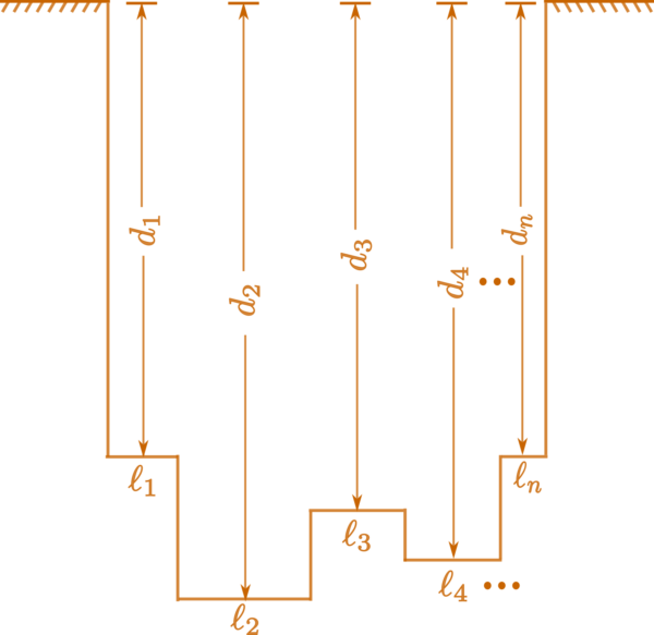
In symbols: If an excavated region of uniform length (but variable depth) comprises n sections of lengths {\ell}_1, \ldots , {\ell}_n and depths d_1, \ldots, d_n respectively (see Figure 1), then the mean depth d of the excavation is defined to be
\[\overline{d}= \frac{{\ell}_1d_1+\cdots+{\ell}_nd_n}{{\ell}_1+\cdots+{\ell}_n}.\]
The mean depth is computed for estimating the volume of the excavation. Just before the quoted line on mean depth, Brahmagupta mentions that the volume of the excavated region is obtained as the area multiplied by its depth. In verses 45–46, he gives a method for estimating the area when the lengths and widths are not uniform.
The brevity that we see in Brahmagupta’s statement is a general feature of the treatises of earlier stalwarts like Āryabhaṭa (499 ce). Detailed expositions were transmitted orally.
Besides, the commentaries are supposed to clarify the statements in the original treatises. Brahmagupta’s verses are explained in the commentary on his treatise by Pṛthūdakasvāmī titled Vāsanā-bhāṣya (c. 864 ce).
3.2 Pṛthūdaka’s Illustrative Example
We quote below an exercise given in Pṛthūdakasvāmī’s commentary to illustrate Brahmagupta’s principle quoted above ([10], p. 136; [18], Vol. III, p. 869; [4], pp. 312–313):
triṁśaddhastā tu yā vāpī dairghyeṇāṣṭau pṛthutvataḥ\,|
tatrāntaḥ pañcakhātāni vedādyairbhuja khaṇḍakaiḥ\,||
vedhaśca navasaptāgatridvisaṅkhyo yathākramam\,|
khātakānāṁ samā rajjuryā’tra syācchīghramucyatām\,||
A pool of water 30 cubits6 in length and 8 cubits in width comprises within it five portions of excavation by which its length is subdivided into (five) parts measuring 4, 5, 6, 7, 8 cubits, the corresponding depths measuring respectively 9, 7, 7, 3, 2 (cubits). Say quickly what is the mean depth of the excavation.
Solution: The areas of the five portions of excavation are (4 \times 9=)\, 36, (5 \times 7=)\, 35, (6 \times 7=)\, 42, (7 \times 3=)\, 21, (8 \times 2=)\, 16 with sum 150 square cubits. Total length is 30 cubits. Therefore, the mean depth is 150 \div 30, i.e., 5 cubits.
The commentary also gives the estimate of the volume of the excavation as the product of its surface area, i.e., (30 \times 8=)\, 240 square cubits, and the mean depth 5 cubits. Thus, the estimated volume is 1200 cubic cubits.
3.3 Śrīdharācārya’s use of Arithmetic Mean in Excavation Problems
In his text Triśatikā (verse 88), Śrīdharācārya (c. 750 ce) presents the following problem on the mean depth of an excavation of uniform length and depth, but variable width ([11], p. 139):
tricatuḥpañcakahastāḥ pṛthutā viṣamāt tu yasya khātasya |
aṣṭau hastā vedho dvādaśa dairghye kathaya phalam ||
In an excavation of uneven width, whose width at (three) different places are 3, 4 and 5 cubits, the depth is 8 cubits and length is 12 cubits. Tell me the volume (of the excavation).
Solution: The mean width is (3+4+5)/3=4 cubits and the estimated volume 12 \times 4 \times 8=384 cubic cubits.
While Brahmagupta introduces weighted arithmetic mean, Śrīdharācārya’s example involves simple arithmetic mean. In section 4.4, we shall see that the formula for weighted arithmetic mean occurs very clearly in Śrīdharācārya’s treatment of mixture problems on gold.
Khāta-vyavahāra (mathematical processes pertaining to excavations) is mentioned in the list of contents of Śrīdharācārya’s longer text Pāṭīgaṇita. It is very likely that in this chapter, Śrīdharācārya had expounded on the concept of weighted arithmetic mean (or at least the arithmetic mean) in the spirit of statistics, as was done by his predecessor Brahmagupta. Unfortunately, this chapter is totally missing from the available manuscript of Pāṭīgaṇita ([19], p. iii).
3.4 Mahāvīrācārya’s Formulation of Arithmetic Mean in Excavation Problems
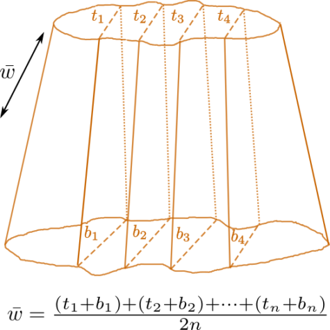
In verse 4 of Chapter 7 of the Gaṇita-sāra-saṅgraha (850 ce), Mahāvīrācārya considers an excavation where the horizontal areas are not constant and moreover, even in any horizontal section, the lengths and widths are not constant (see Figure 2). Mahāvīrācārya applies a “midpoint” type rule. Consider n vertical sections of the excavation along its length; and measure the length of the top and the length of the bottom of each vertical section. Consider the half of the sums of these n estimates of the lengths of the face and the base. Mahāvīrācārya prescribes taking the mean length as the above (halved) number divided by the number n. Thus, if t_1, t_2, \ldots, t_n are the top-lengths and b_1, \ldots, b_n are the corresponding bottom-lengths, then the mean length is given by \left((t_1+b_1)+\cdots+(t_n+b_n)\right)/2n. Similarly, one gets the mean width. The product gives an estimate of the area. A working estimate of the volume of the excavation is given by the product of this estimated area with the depth.
The verse of Mahāvīrācārya is ([14], p. 143 (Sanskrit); p. 258 (English)):
kṣetraphalaṁ vedhaguṇaṁ samakhāte vyāvahārikaṁ gaṇitam |
mukhatalayutidalamatha satsaṅkhyāptaṁ syātsamī karaṇam ||
The usual measure (i.e., the volume) of a regular excavation is given by the product of its area and its depth. Now (to obtain a working estimate of the dimensions, i.e., length and width, of an irregular excavation), take the half of the sums of the top and bottom (dimensions, i.e., lengths, resp. widths) and divide (the halved number) by the number (of sections). That is the mean (length, resp. width, of the excavation).
Mahāvīrācārya gives several numerical exercises on excavation.
3.5 Bhāskarācārya’s Formulation of Arithmetic Mean in Excavation Problems
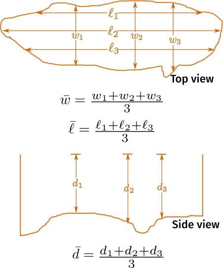
The statistical arithmetical mean is lucidly described by Bhāskarācārya in his treatise Līlāvatī in the context of estimating the volume of an excavation when all three dimensions vary (see Figure 3). However, he does not adopt any “midpoint” type rule. Bhāskarācārya says ([12], p. 151; [16], p. 145):
gaṇayitvā vistāraṁ bahuṣu sthāneṣu tadyutirbhājyā\,|
sthānakamityā samamitirevaṁ dairghye ca vedhe ca
kṣetraphalaṁ vedhaguṇaṁ khāte ghanahastasaṅkhyā syāt\,||
The width of the ditch is to be measured at several places. The mean width of the ditch is defined to be the quotient of the sum of the widths divided by the number of places (at which the measurements are taken). Likewise, the mean length and mean depth are determined. Then the estimated volume of the ditch will be the product of the estimated area (obtained as the product of the mean length and the mean breadth) and the mean depth.
In the next verse ([12], p. 151; [16], p. 146), Bhāskarācārya sets the following exercise on computing the volume of an irregular shape:
bhujavakratayā dairghyaṁ daśeśārkakarairmitam |
triṣu sthāneṣu ṣaṭpañcasaptahastā ca vistṛtiḥ ||
yasya khātasya vedho’pi dvicatustrikaraḥ sakhe |
tatra khāte kiyantaḥ syurghanahastāḥ pracakṣva me ||
Taking measurements of the curved sides of an irregular ditch at three places, the lengths obtained are 10, 11 and 12 cubits; breadths 6, 5 and 7 cubits; and depths 2, 4 and 3 cubits. O friend! Tell me the volume of the ditch in cubic cubits.
Here, mean length in cubits is (10+11+12)\div 3=11, mean breadth is (6+5+7)\div 3=6 and mean depth is (2+4+3) \div 3=3. By Bhāskarācārya’s principle, the estimated volume is (11 \times 6)\times 3=198 cubic cubits.
In his treatise Gaṇita Kaumudī (c. 1350 ce), Nārāyaṇa Paṇḍita too makes a statement similar to that of Bhāskarācārya on the mean width, length or depth of an irregular excavation and on the consequent estimation of its volume; it is followed by a numerical exercise ([21], p.21).
3.6 Gaṇeṣa Daivajña’s Heuristic Version of the Law of Large Numbers
In his commentary on Līlāvatī titled Buddhivilāsinī (c. 1545 ce), Gaṇeṣa Daivajña makes the following remark ([16], p. 145) while explaining Bhāskarācārya’s verses on measuring irregular shapes quoted above.
yathā yathā bahuṣu sthāneṣu vistārādikaṁ gaṇyate
tathā tathā samamitiḥ sūkṣmasūkṣmatarā syāditi spaṣṭam |
The more and more the number of places at which the measurements of width, etc., are taken, the closer and closer will the mean measures be to the true values and [consequently] the computation [of the volume] will be more and more accurate.
The Law of Large Numbers, a basic pillar of the theory of probability, states that the sample mean converges to the distribution mean (i.e., the true mean) as the sample size increases. A mathematically precise version of this fundamental principle was stated and proved by Jacob Bernoulli (1654–1705) in his seminal treatise Ars Conjectandi (The Art of Conjeturing), published posthumously in 1713 ce. A rudimentary form of the law is implicit in a statement of G. Cardano (1501–76) in his Liber de Ludo Aleae (The Book on Games of Chance), written around 1563 ce and published posthumously in 1663 ce. The statement of Gaṇeṣa can be considered an explicit heuristic formulation of the law of large numbers.7
3.7 The Seeds of Calculus in Arithmetic Mean
We share below a few thought-provoking comments (in private communication) from two mathematicians in response to the article [7].
David Mumford8 writes that while the topic “finite differences” was one stepping stone towards the invention of calculus in India, the article [7] makes it clear that the “Arithmetic Mean” was another.
Avinash Sathaye9 points out that the idea of approaching the correct area (or volume) of a region by increasing the subdivisions of the region, that is explicitly stated by Gaṇeṣa, is analogous to the idea of Riemann Sums in integral calculus. Sathaye also remarks that this idea of using separate (arithmetic) means for the three dimensions can be seen in the light of the Mean Value Theorem of integral calculus; indeed, it is a special case of the latter.
Recall that, by the Mean Value Theorem for a smooth function f, \int_{a}^{b} f(t)dt=(b-a)M, where M is the so-called mean value. As the very name suggests, this mean value M is a generalization of the Arithmetic Mean. If we consider a rectangle whose base is b-a and whose area is the same as the area under the curve defined by f, then M equals the height of the rectangle. If the interval [a,b] is divided into n equal pieces, and M_i is the height of the rectangle with area same as the area under the curve over the ith sub-interval, then M is precisely the Arithmetic Mean of the heights M_i‘s.
4 Weighted Arithmetic Mean in Ancient India: Computations on the Purity of Gold in Alligation Problems
4.1 The Terms varṇa, kṣaya and māṣa
The word fineness is used to indicate the proportion of a pure precious metal in an alloy of the metal. The Sanskrit word varṇa, whose meanings include “colour”, “lustre”, “glory”, “quality”, etc., is used in ancient Indian treatises to denote the “fineness” (or purity) of gold; the fineness of pure gold is defined to be 16 varṇa. Thus, a gold of 1 varṇa contains 1 part of pure gold and 15 parts of impurities (in the form of baser metals); a gold of 2 varṇa contains 2 parts of pure gold and 14 parts of impurities, and so on. The term varṇa is thus analogous to the modern term karat (also spelt as carat), with pure gold being 24 karat, i.e., 16 varṇa = 24 karat.
Just as varṇa (lustre) indicates the purity of gold, the term kṣaya (usual meanings: diminution, loss, etc.) has been used in certain texts to indicate the deficiency (i.e., the proportion of impurities) in a piece of gold; a gold of 1 kṣaya contains 1 part of impurities and 15 parts of pure gold; a gold of 2 kṣaya contains 2 parts of impurities and 14 parts of pure gold, and so on. Thus, if a piece of gold is of fineness v varṇa and deficiency k kṣaya, then v+k=16 (cf. [19], p. 38 (English)).
A traditional Indian unit for the weight of gold is a māṣa (approximately, 0.97 gram). Some of the Sanskrit synonyms for gold like hema, suvarṇa (literally, “having good (or beautiful) colour”), kanaka, svarṇa are also used for the weight of a piece of gold. Further, some of these terms are also used as specific units for the weight of gold: for instance, a piece of gold of weight 16 māṣa is called suvarṇa ([19], p. 5 (Sanskrit); [15], p. 5).
Note that the amount of pure gold in a piece of gold of weight w units and fineness v varṇa is (wv)/16 units.
4.2 Alligation and Weighted Arithmetic Mean
One of the standard topics in ancient Indian arithmetic treatises is miśraka-vyavahāra (alligation, i.e., computations pertaining to mixtures of things). A central problem on alligation is the computation of the fineness of a piece of gold formed by combining several pieces of gold of different weights and purities.
The formula for weighted arithmetic mean arises very naturally in some of these problems on alligation: if n pieces of gold of fineness v_1, \ldots, v_n varṇa and weights w_1, \ldots, w_n units are combined, then the fineness of gold in the resultant piece is V varṇa, where
\[\begin{equation}\label{eq1}
V= \frac{w_1v_1+\cdots+w_nv_n}{w_1+\cdots+w_n}. \tag{4.1}
\end{equation}\]
Thus, V is literally the “weighted” arithmetic mean of the fineness of the original pieces, with the literal weight of the gold pieces playing the role of the mathematical weight.
As we shall see in this section, the formula \(\eqref{eq1}\) is described, with numerical examples, in several ancient Indian treatises. The proof of the relation \(\eqref{eq1}\) can be seen by equating the amount of pure gold in an alloy of V varṇa of weight w_1+\cdots+w_n units [i.e., \left(V(w_1+\cdots+w_n)\right)/16 units] with the sum of the amounts of pure gold in alloys of v_i varṇa of weights w_i [i.e., (w_1v_1+\cdots +w_nv_n)/16 units].
However, note that when different pieces of gold are mixed up, melted and refined, the weight of the refined gold need not, in reality, be the sum of the weights of the components as some of the impurities could get burnt out during the process of refinement. Suppose that n pieces of gold of weights w_1, \ldots, w_n units with respective fineness v_1, \ldots, v_n varṇa are mixed up, melted and refined. Let the weight of the refined gold be w units and its fineness be v varṇa. The difference w_1+\cdots+w_n -w would be the amount of impurities that get burnt out during the process of refinement. The refinement process does not involve any change in the amount of pure gold. Therefore, equating the amount of pure gold in the aggregate of the original pieces [i.e., (w_1v_1+\cdots +w_nv_n)/16 units] with the amount of pure gold in the new piece [i.e., (vw)/16 units], we see the following relation between the fineness and the weight of the refined gold:
\[\begin{equation}\label{eq2}
v= \frac{w_1v_1+\cdots+w_nv_n}{w}. \tag{4.2}
\end{equation}\]
Along with the statement \(\eqref{eq1}\) on weighted A.M., ancient Indian texts also mention this modified formula.
Now suppose that one wishes to form, from the initial pieces of gold, a new piece of gold of a certain specified varṇa v^{\prime} (by suitably adjusting the amount of impurities). Arguing as before, it can be seen that the weight w^{\prime} of the required piece of gold will then be
\[\begin{equation}\label{eq3}
w^{\prime}= \frac{w_1v_1+\cdots+w_nv_n}{v^{\prime}}, \tag{4.3}
\end{equation}\]
which is, mathematically, a rephrasing of rule \(\eqref{eq2}\). Indian authors explicitly mention this rule too.
Below, we make a brief reference to the application of weighted arithmetic mean in the ancient Indian treatise named “Bakṣālī Manuscript” (c. 300 ce).10
4.3 Weighted Arithmetic Mean in the Bakṣālī Manuscript
The weighted arithmetic mean is defined in H1 16 verso (ii) of the Bakṣālī Manuscript, in the context of computing the kṣaya of gold in a mixture. The statement in the manuscript is ([17], p. 46):
kṣayaṁ saṁguṇya kanakāstadyutirbhājayet tataḥ
saṁyutaireva kanakairekaikasya kṣayo hi saḥ
Having multiplied the [weights of the] pieces of gold with their kṣaya, let their sum (i.e., the sum of the products) be divided by the sum of the [weights of the] pieces of gold. The result is the average kṣaya.
Thus, if n pieces of gold of weights w_1, \ldots, w_n units have respective kṣaya k_1, \ldots, k_n, then the average kṣaya is given by
\[k=\frac{w_1k_1+\cdots+w_nk_n}{w_1+\cdots+w_n}.\]
Two numerical examples are worked out as illustrations ([17], pp. 46–47). In the first example [H1 (16 verso) (iii)], n=4, k_1=1, k_2=2, k_3=3, k_4=4 and w_1=1, w_2=2, w_3=3, w_4=4. Thus, the average kṣaya
\[k=\frac{1\times 1+2\times 2+3\times 3+4 \times 4}{1+2+3+4}=\frac{30}{10}=3.\]
In the second example [H2 (17 recto., 17 verso) (ii)], n=4, w_1=1, w_2=2, w_3=3, w_4=4 māṣa and k_1=\frac{1}{2}, k_2=\frac{1}{3}, k_3=\frac{1}{4}, k_4=\frac{1}{5} kṣaya. Thus, the average kṣaya
\[k=\frac{1\times \frac{1}{2}+2\times \frac{1}{3}+3\times \frac{1}{4}+4 \times \frac{1}{5}}{1+2+3+4}=\frac{163}{600}.\]
It then appears that, within 300 CE, the weighted arithmetic mean had arisen in ancient India as an exact mathematical concept, from mixture problems involving computations on gold. From the early seventh century, the weighted arithmetic mean was conceived in its statistical avatar by Brahmagupta and subsequent Indian mathematicians, and applied (somewhat in the spirit of calculus) to problems involving estimation of the dimensions of an excavation.
We now quote some of the statements in ancient Indian texts on the three rules \(\eqref{eq1}\), \(\eqref{eq2}\) and \(\eqref{eq3}\). There are several other formulae on alligation in these texts which are not being mentioned in our present article. Some of these problems are algebraic: for instance, the problem of finding the unknown fineness or the unknown weight of one of the components from the data about the mixture and its other components.
4.4 Śrīdharācārya’s Formulation of the Weighted A.M. for Alligation
In his treatise Pāṭīgaṇita, Śrīdharācārya states the rule \(\eqref{eq1}\) in the following words ([19], p. 63):
hemaguṇavarṇayoge hemaikyahṛte bhavedvarṇaḥ ||
The sum of the products of weight and fineness of (several pieces of) gold, divided by the sum of the weights (of those pieces) of gold, shall become the fineness (of the resultant piece).
The same principle is also stated in different words in Triśatikā ([11], p. 88). Both texts mention two similar numerical examples as exercises on the above principle; there are slight differences in the numerical data in the two versions. The first exercise in Pāṭīgaṇita is ([19], p. 63):
dvādaśadaśakaikādaśavarṇakanavapañcasaptadaśa māṣāḥ |
kanakasya samāvarte jāyante varṇake kasmin ||
When gold pieces of fineness 12, 10, and 11 varṇa with respective weights 9, 5, and 17 māṣa are combined (i.e., melted together), what is the fineness of the produced gold?
The solution is given in an ancient commentary ([19], p. 63) as follows. The products of the weight and the fineness of the gold pieces are 9 \times 12=108, 5 \times 10=50 and 17 \times 11=187. The sum of these three products is (108+50+187=) 345. The sum of the weights is (9+5+17=) 31. On division, the resultant fineness in varṇa is \left(\frac{345}{31}=\right) 11 {\small \frac{4}{31}}.
In the version in Triśatikā ([11], p. 89), the weight of the third gold piece is given to be 16 instead of 17; in this case, the resultant fineness will be 11 {\small \frac{2}{15}} varṇa.
We now quote the second exercise from Pāṭīgaṇita ([19], p. 63), rectifying a spelling error.11
sārdhaikādaśadaśakārdhāṣṭamavarṇāḥ kvavarṇake yogāt |
tryaṁśaṣaḍaṁśārdhānvitapañcacatussaptamāṣāḥ syuḥ ||
What is the fineness [of the gold piece obtained] when [three gold pieces of] 11 \small{\frac{1}{2}}, 10 and 7 \small{\frac{1}{2}} varṇa [with respective weights] 5 \small{\frac{1}{3}}, 4 \small{\frac{1}{6}}, 7 \small{\frac{1}{2}} māṣa are combined [into one]?
The solution is given in the ancient commentary ([19], p. 64) as follows. The products of the weights and the fineness of the gold pieces are \frac{16}{3} \times \frac{23}{2}=\frac{368}{6}, \frac{25}{6} \times 10=\frac{250}{6} and \frac{15}{2} \times \frac{15}{2}=\frac{225}{4}. The sum of these three products is \frac{1911}{12}=\frac{637}{4}. The sum of the weights is \frac{102}{6}=17 māṣa. On division, the fineness comes out as \frac{637}{68}= 9 {\small \frac{25}{68}} varṇa.
In the version in Triśatikā ([11], p. 90), the weight of the first gold piece is given to be 5 \small{\frac{1}{2}} instead of 5 \small{\frac{1}{3}}; the final answer in this case will be 9 {\small \frac{40}{103}} varṇa.
The modified formula \(\eqref{eq2}\) is stated by Śrīdharācārya in both Pāṭīgaṇita ([19], p. 64) and Triśatikā ([11], p. 90) in the following words:
varṇasuvarṇavadhaikyaṁ vipakvakanakena bhājitaṁ varṇaḥ
The sum of the products of the fineness and the (weights of several pieces of) gold, divided by the (weight of the) refined gold, becomes the fineness (of the refined gold).
The following exercise is set in both the texts ([11], p. 91; [19], p. 64):
pañcāṣṭaṣaṭsuvarṇā dvādaśanavakārdhapañcadaśavarṇāḥ\,|
pakvāḥ ṣoḍaśa dṛṣṭāstad varṇaka ucyatāmāśu\,||
Gold pieces of weights 5, 8 and 6 suvarṇa and respective fineness 12, 9 and (15-\frac{1}{2}=) 14 \frac{1}{2} varṇa, mixed together and refined, are seen to reduce to 16 suvarṇa in all. Quickly state the varṇa of the refined gold.
Note that the sum of the weights of the original pieces is 19 suvarṇa; thus there has been a reduction of 3 suvarṇa during the process. The ancient commentary discusses the problem in detail ([19], pp. 64–66) and gives the final answer \frac{219}{16}. The commentary also points out that the weighted mean of the varṇas of the original pieces is \frac{219}{19}.
In Pāṭīgaṇita ([19], p. 66) as well as Triśatikā ([11], p. 90–91), Śrīdharācārya describes the formula \(\eqref{eq3}\) and a numerical exercise on it.
4.5 Mahāvīrācārya’s Version of Weighted A.M. in Alligation
Mahāvīrācārya states the rules \(\eqref{eq1},\eqref{eq2}\) in a condensed form in the first part of verse 169 of Gaṇita-sāra-saṁgraha as follows ([14], p. 87):
kanakakṣayasaṁvargo miśrasvarṇāhṛtaḥ kṣayojñeyaḥ |
Mahāvīrācārya then gives a numerical example (in verses 170–171.5), where the formula \(\eqref{eq1}\) on weighted A.M. has to be employed. This is followed by his statement of rule \(\eqref{eq3}\) and two numerical examples on it.
We mention here that one of the problems stated by Mahāvīrācārya in his chapter on mixture problems (268.5, 273.5) is an example of what is now termed as a “Dutch bet”, i.e., a rule in gambling which ensures profit for a particular person irrespective of his victory or loss. The “Dutch bet” and Mahāvīrācārya’s problem are often mentioned by authors discussing the history of probability. (For instance, see [9], p. 8.)
4.6 Pṛthūdakasvāmī’s Supplement
In his commentary on the chapter Gaṇitādhyāyaḥ of the treatise Brāhma Sphuṭa Siddhānta (628 ce) by Brahmagupta, Pṛthūdakasvāmī (c. 864 ce) points out that the topic of computations on gold does not occur in the chapter and therefore, he introduces a verse of his own on the omitted topic. Pṛthūdaka says ([10], p. 70):
iha gaṇitādhyāye suvarṇagaṇitaṁ nāsti |
tadartha śloko’yam
His rule describes the formulae \(\eqref{eq3}\) and \(\eqref{eq1}\):
suvarṇahemasaṁvargānekīkṛtya vibhājayet |
iṣṭavarṇena tatsaṅkhyā hemayogena varṇakaḥ ||
Take the sum of the products of the fineness and the weight of the several pieces of gold. Dividing it by the fineness of the desired (refined gold) gives the amount (the weight of the refined gold); dividing it by the sum of the weights of the (pieces of) gold gives the fineness (of the refined gold).
Pṛthūdaka illustrates his rule with an example ([4], p. 289) involving three pieces of gold: one of weight 5 suvarṇa and fineness 12 varṇa, one of weight 6 suvarṇa and fineness 13 varṇa, and one of weight 7 suvarṇa and fineness 14 varṇa. Thus, the sum of the products is 60+78+98=236. If the resultant fineness is 16 varṇa, then the amount of gold in the mixture is \frac{236}{16} suvarṇa, i.e., 14 suvarṇa and 12 māṣa. The fineness is given by \frac{236}{18}, i.e., 13 \small{\frac{1}{9}} varṇa.
4.7 Bhāskarācārya’s Formulation of the Weighted Arithmetic Mean in Alligation
In the following verse ([12], p. 97; [15], p. 182), Bhāskarācārya makes a compact and lucid presentation of the rules \(\eqref{eq1}\), \(\eqref{eq2}\) and \(\eqref{eq3}\) in his treatise Līlāvatī. The first line prescribes the formula for weighted arithmetic mean \(\eqref{eq1}\); the next line is on rules \(\eqref{eq2}\) and \(\eqref{eq3}\).
suvarṇavarṇāhatiyogarāśau svarṇaikyabhakte kanakaikyavarṇaḥ |
varṇo bhavecchodhitahemabhakte varṇoddhṛte śodhitahemasaṅkhyā ||
The sum of the products of the weights and the fineness of the (pieces of) gold, divided by the sum of the weights of the (pieces of) gold, defines the fineness of the mixture of the gold pieces. The sum, divided by the weight of the purified gold, defines the fineness of the purified gold; and (the sum) divided by the fineness of the purified gold, defines the amount (weight) of the purified gold.
Bhāskarācārya has indicated that the above results follow from the well-known inverse rule of three in arithmetic. In an earlier verse of Līlāvatī, Bhāskarācārya has emphasized that this rule has applications in problems involving quantities which are inversely related, i.e., where the increase of one quantity results in the decrease of the other and vice versa. He then gives the following examples where the inverse rule of three is to be applied ([12], p. 81; [15], p. 137):
jīvānāṁ vayaso maulye taulye varṇasya hemani |
bhāgahāre ca rāśīnāṁ vyastaṁ trairāśikaṁ viduḥ12 ||
In (problems involving) the age of living beings and their value,13 the weight and fineness of objects of gold, the division of heaps (of grain),14 the use of the inverse rule of three is well-known.
After his verse stating rules \(\eqref{eq1}\), \(\eqref{eq2}\) and \(\eqref{eq3}\), Bhāskarācārya gives an exercise in two parts in his next two verses. The two parts correspond to the two parts of his theorem on the three rules. The first verse, quoted below, is on the rule \(\eqref{eq1}\) on weighted arithmetic mean ([12], p. 98; [15], p. 183):
viśvārkarudradaśavarṇasuvarṇamāṣā digveda
locanayugapramitāḥ krameṇa |
āvartiteṣu vada teṣu suvarṇavarṇastūrṇaṁ suvarṇagaṇitajña vaṇigbhavetkaḥ ||
(Four types of gold pieces of) fineness 13, 12, 11 and 10 varṇa, and weights 10, 4, 2 and 4 māṣa respectively, are melted together. Tell me quickly O merchant, thou expert on the mathematics of gold (or golden mathematician), what will be the fineness of the (new piece of) gold?
The formula \(\eqref{eq1}\) described by Bhāskarācārya gives the fineness
\[
\begin{equation*}
\frac{(10 \times 13)+(4 \times 12)+(2 \times 11)+(4 \times 10)}{10+4+2+2}=\frac{240}{20} =12
\end{equation*}
\]
In his commentary on Līlāvatī titled Buddhivilāsinī (c. 1545 ce), Gaṇeṣa Daivajña explains the solution in detail. Instead of applying the formula \(\eqref{eq1}\) straightaway, Gaṇeṣa works out the solution from first principles, making an implicit application of the “Inverse Rule of Three”. Gaṇeṣa’s exposition provides, in essence, a proof of the principles \(\eqref{eq1}\) and \(\eqref{eq2}\). As the passage is long ([15], p. 185–186), we summarize below its essential content.
Solution (Gaṇeṣa Daivajña): The fineness and the weight are in inverse proportion.
Suppose the fineness of all the gold pieces becomes 1 varṇa. Then the weight of the first piece (of original fineness 13 varṇa and weight 10 māṣa) becomes (13 \times 10=)\, 130 māṣa. Similarly, the weights of the remaining three pieces of gold (of original weights 4, 2 and 4 māṣa) become (12 \times 4=)\, 48, (11 \times 2=)\, 22 and (10 \times 4=)\, 40 māṣa.
Hence the total weight of the original pieces of gold in an alloy of fineness 1 varṇa would be 130+48+22+40= 240 māṣa. Therefore, for 20 \,(=10+4+2+4) māṣa, the fineness of gold has to be \left(\frac{240 \times 1}{20}=\right)\, 12 varṇa.
The next verse of Bhāskarācārya gives the second part of his exercise on rules \(\eqref{eq2}\) and \(\eqref{eq3}\). He asks ([15], p. 184):
te śodhanena yadi ca viṁśatiruktamāṣāḥ syuḥ ṣoḍaśā”śu vada varṇamitistadā kā |
cecchodhitaṁ bhavati ṣoḍaśavarṇahema te viṁśatiḥ kati bhavanti tadā tu māṣāḥ ||
If the 20 māṣa (of gold) mentioned above reduces to 16 when refined, tell me quickly what will be the fineness (of the refined gold). On the other hand, if, on purification, it becomes gold of 16 varṇa, then what is the number of māṣa to which the 20 māṣa will become reduced?
Solution: In the first case, by formula \(\eqref{eq2}\), the fineness of the refined gold will be \left(\frac{240}{16}=\right)\, 15 varṇa. In the second case, by formula \(\eqref{eq3}\), the weight of the refined gold will be \left(\frac{240}{16}=\right)\, 15 māṣa. In the first case, 4 māṣa of impurities got burnt out; in the second case, 5 māṣa of impurities got burnt out.
A similar statement and exercise on alligation as that of Bhāskarācārya is also given by Nārāyaṇa Paṇḍita ([20], p.60).
5 Influence of Ancient Indian Arithmetic and Algebra
We now offer a few possible explanations for the early occurrence of the general Arithmetic Mean in ancient India and its delayed introduction in Europe. The history of modern arithmetic appears to hold a key.
5.1 The Impact of the Decimal System and the Operation of Division
The decimal system originated in India. In spite of the strong advocacy by Fibonacci (c. 1202 ce) and subsequent scholars, it took nearly five centuries for the Indian decimal system to get accepted and standardized in Europe, sometime around the 17th century. Till then, Roman numerals were in use. The eventual adoption of the decimal system is considered one of the factors for the mathematical and scientific renaissance in Europe.15
Thanks to the decimal system, ancient Indians could develop neat and systematic methods for fundamental arithmetic operations like addition, subtraction, multiplication, division. Their methods were slight variants of our current methods.16 For instance, a variant of the modern method of “long division” had become firmly established in India well before the 5th century. It is a crucial component of the ingenious algorithms of Āryabhaṭa (499 ce) for computing square roots and cube roots (which are again slight variants of the present methods). By contrast, the methods of computation based on the Roman system practised in Europe were unwieldy. The decimal system brought an enormous simplification in computational arithmetic in Europe.
Now, the computation of Arithmetic Mean involves the operation of division (apart from multiplication and addition) and, for a long time (till at least the 15th century), division was regarded as a difficult operation by European scholars. As late as in 1494 ce, Luca Pacioli had remarked, “if a man can divide well, everything else is easy, for all the rest is involved therein” ([22], p. 132). Not much is known about ancient European methods of division other than the process of repeated subtraction. The Indian version of long division went to Europe through the Arabs and became very popular during the 15th–18th centuries as the galley method. Some modifications were subsequently introduced to make it conducive for the new system of writing with paper-and-ink.17
Thus, it is perhaps not a coincidence that we see an increasing use of the Arithmetic Mean in Europe after her adaptation of the Indian computational methods based on the decimal system.
The occurrence of a chapter “on mixture” (De’ mescolo) in early Italian works on arithmetic was probably influenced by the miśraka-vyavahāra chapter in ancient Indian texts ([5], p. 233).
5.2 The Impact of Algebra
We may find it incredible that although the ancient Greeks had defined Arithmetic Mean for two numbers, it would take around two thousand more years for the idea of A.M. of n numbers to emerge in Europe. The catch here seems to be that today, with our training in algebra from an early age, we tend to think of A.M. for two numbers as “(a+b)/2” and hence find “(a_1+ \cdots + a_n)/n” a natural generalization. But the very formulation “(a_1+ \cdots + a_n)/n” is something intrinsically algebraic (whether expressed through symbols or words). And so is the idea of generalizing from 2 to an arbitrary n. As emphasized in section 2.1, the Greek A.M. was essentially a geometric concept, the mid-point of the line segment joining two points.18
The subject “Algebra” had come out explicitly in the open in ancient India by the time of Brahmagupta (628 ce); many of its features can already be seen in the the Bakṣālī Manuscript (c. 300 ce) and the work of Āryabhaṭa (499 ce). Thus, along with the decimal system and arithmetic, the algebra culture too must have provided a conducive environment for the emergence of the Arithmetic Mean in ancient India.
6 Epilogue
We have seen in section 3 that, from at least the 7th century ce, Indian mathematicians have not only defined the Arithmetic Mean explicitly, not only given the concept an appropriate name, but have also treated it as a representative value. For instance, conceptually, Brahmagupta’s representation of the depth of an irregular ditch (of variable depth) by the Arithmetic Mean of the depths at various places is not the case of taking an average of repeated measurements of the same quantity to reduce errors of measurement; rather, it is an early example of taking the mean depth as a representative value among genuinely different values. This statistical concept occurs in the major texts of prominent astronomer-mathematicians like Brahmagupta and Bhāskarācārya, whose English translations [4] have been available for the past 200 years.
And yet, the abundant occurrence of Arithmetic Mean in ancient Indian mathematics texts gets overlooked in accounts on history of statistics. Should we in India cling to our culture of cultivated ignorance about ancient Indian science?
We end the article with a remark of David Mumford to the author in the context of the article [7]. Mumford observes that it is interesting that “dirt and gold were the two applications” of the Arithmetic Mean in India. Perhaps that is symbolic of the yogic equality in Indian spiritual tradition, or the expression ṭākā māṭi māṭi ṭākā (money is mud, mud is money) of Sri Ramakrishna!
acknowledgements I thank all the readers of [7] for their enthusiastic responses and for pointing out the typing errors. I especially thank Avinash Sathaye for several corrections and improvements in the translations of the Sanskrit verses.
References
- [1] P.C. Mahalanobis. Sankhyā. 1933. 1(1): 1–4
- [2] P.C. Mahalanobis. Why Statistics?. Sankhyā. 1950. 10(3): 195–228
- [3] Arthur Bakker and Koeno P.E. Gravemeijer. An Historical Phenomenology of Mean and Median.Educational Studies in Mathematics. 2006. 62: 149–168
- [4] H.T. Colebrooke. Algebra, with Arithmetic and Mensuration, from the Sanscrit of Brahmegupta and Bhascara. John Murray, London (1817); reprinted Cosmo Pub (2004); Sharada (2005)
- [5] Bibhutibhusan Datta and Avadhesh Narayan Singh. History of Hindu Mathematics Part I. Motilal Banarasidass (1935); reprinted by Asia Publishing House (1962) and Bharatiya Kala Prakashan (2004)
- [6] A.K. Dutta. The bhāvanā in Mathematics. Bhāvanā. 2017. 1(1): 13–19
- [7] A.K. Dutta. The Concept of Arithmetic Mean in Ancient India, in 25 Years Gone By (ed. A. Chaudhuri). ISIREA (2017): 158–192
- [8] Churchill Eisenhart. The Development of the Concept of the Best Mean of a Set of Measurements from Antiquity to the Present Day. American Statistical Association Presidential Address. 1971. http://galton.uchicago.edu/ stigler/eisenhart.pdf
- [9] Ian Hacking. The Emergence of Probability: A Philosophical Study of Early Ideas about Probability, Induction and Statistical Inference. Cambridge University Press. 1975
- [10] V.D. Heroor (tr.) Brahmaguptagaṇitam. Chinmaya International Foundation Shodha Sansthan, Ernakulam. 2014
- [11] V. Kutumbashastri (ed.) and Sudyumnacharya (Hindi tr.) The Pātigaṇitasāra of Srīdharācārya. Rashtriya Sanskrit Sansthana. 2004
- [12] K.S. Patwardhan, S.A. Naimpally and S.L. Singh (eds.) Līlāvatī of Bhāskarācārya. Motilal Banarasidass. 2001
- [13] R.L. Plackett. The Principle of the Arithmetic Mean, in Studies in the History of Statistics and Probability. 1 (eds. E.S. Pearson and M.G. Kendall). Griffin, London. 1970: 121–126
- [14] M. Raṅgācārya (ed. with English translation and notes).The Gaṇita-sāra-saṅgraha of Mahāvīrācārya. Govt. of Madras, Madras. 1912
- [15] A. Padmanabha Rao. Bhāskarācārya’s Līlāvatī Part I. Chinmaya International Foundation Shodha Sansthan, Ernakulam. 2015
- [16] A. Padmanabha Rao. Bhāskarācārya’s Līlāvatī Part II. Chinmaya International Foundation Shodha Sansthan, Ernakulam. 2014
- [17] Svami Satya Prakash Sarasvati and Usha Jyotishmati (ed.) The Bakshali Manuscript. Dr. Ratna Kumari Svadhyaya Sansthana, Allahabad. 1979
- [18] R.S. Sharma (ed.) Brāhma Sphuṭa Siddhānta of Brahmagupta. Indian Institute of Astronomical Research. 1966
- [19] K.S. Shukla (ed.) The Patiganita of Sridharacarya. Lucknow University. 1959
- [20] Paramanand Singh (ed.) The Gaṇita Kaumudī of Nārāyaṇa Paṇḍita. Gaṇita Bhāratī. 1998. 20: 25–82
- [21] Paramanand Singh (ed.) The Gaṇita Kaumudī of Nārāyaṇa Paṇḍita Chapters V–XII. Gaṇita Bhāratī. 2000. 22: 19–85
- [22] D.E. Smith. History of Mathematics. II. Dover. 1958 (originally 1925).
- [23] Stephen M. Stigler. The History of Statistics. Harvard University Press. 1986
- [24] Stephen M. Stigler. The Seven Pillars of Statistical Wisdom. Harvard University Press. 2016
Footnotes
- Stephen M. Stigler (b. 1941), a student of Lucien Le Cam, is a distinguished statistician at the University of Chicago, known for his work on the history of statistics. ↩
- In his paper “Probability in Ancient India” (in Handbook of the Philosophy of Science. (eds. P.S. Bandyopadhyay and M.R. Forster). Elsevier. 2010. 7: 1171–1192), C.K. Raju does mention the occurrence of weighted A.M. in the works of Śrīdharācārya and others in the context of mathematical computations on the density of gold; but even his account overlooks the much earlier statistical use of the weighted A.M. by Brahmagupta. ↩
- The term used was “centre of gravity”. ↩
- Gauss mentions that he was aware of the method since 1795 (see [23], p. 15). ↩
- From the English translation by C.H. Davis of Theoria motus corporum coelestium in sectionibus conicis solem ambientium (Theory of the motion of the heavenly bodies moving about the sun in conic sections) by C.F. Gauss; quoted by G.B. Rossi in “Probability in Metrology”, in Data Modeling for Metrology and Testing (eds. F. Pavees and A.B. Forbes). Birkhauser. 2009. p. 34. ↩
- A “cubit” is an ancient unit of length of around 18 inches, based on the length of the forearm from the tip of the middle finger to the base of the elbow. In Sanskrit, the cubit is called hasta or kara (literally, the forearm). ↩
- Oscar Sheynin makes a reference to this statement of Gaṇeṣa, as translated by Colebrooke ([4], p. 97), in his paper “On the Early History of the Law of Large Numbers”. Biometrika. 1968. 55(3): 459.↩
- David Mumford (b. 1937), a student of Oscar Zariski, is a distinguished mathematician who was awarded the Fields Medal (1974) for his contributions to algebraic geometry. Mumford has had a profound influence on Indian algebraic geometers. His books Abelian Varieties (with C.P. Ramanujam) and Tata Lectures on Theta were based on his lectures at TIFR. (A picture of TIFR occurs in the cover of the reprint of the book Abelian Varieties.) Mumford is also noted for his work in pattern theory and computer vision, and his deep interest in history of mathematics, including ancient Indian mathematics. He is now at Brown University, USA. ↩
- Avinash Sathaye (b. 1948), a student of S.S. Abhyankar, has made fundamental contributions in several areas of algebra and affine algebraic geometry, including the study of complete intersections, affine spaces and affine fibrations. The works of several Indian algebraists have been the offshoots of his pioneering results. Sathaye is also a Sanskrit scholar and an authority on history of mathematics. He is now at the University of Kentucky, USA. ↩
- Historians of mathematics differed in their estimates of the date of this work but a recent radiocarbon dating of the text at the University of Oxford’s Bodelian Libraries supports the view of scholars like B. Datta that the original version of the treatise was composed around the third century ce or earlier. ↩
- The editor K.S. Shukla notes that the only available manuscript “is full of errors and inaccuracies” ([19], p. (iii)). ↩
- In some versions, the word bhavet occurs in place of viduḥ. ↩
- In this verse, there is an underlying assumption that older the living being, lesser is the capacity for work and other qualities and therefore, lesser is the utility (value) and hence lesser is the wage (in case of human beings) or price. ↩
- The bigger the size of a measure by which the heap is measured, the smaller will be the number of measures. ↩
- For details on the history and transmission of the decimal system, see the articles “Decimal System in India” by A.K. Dutta in Encyclopaedia of the History of Science, Technology, and Medicine in Non-Western Cultures (ed. H. Selin). Springer. 2016. pp. 1492–1504; and “Spread and Triumph of Indian Numerals” by R.C. Gupta in Indian J. History of Science. 1983. 18(1): 23–38. ↩
- In fact, etymologically, the word “algorithm” is related to ancient Indian arithmetic. As the Indian decimal system and computational arithmetic was expounded by Al-Khwārizmī (c. 820 ce), operations based on the decimal system acquired the name algorismus, derived from Algoritmi, the Latin form of Al-Khwāarizmī. Thus emerged “algorism”, which later became “algorithm”! The original Indian algorithms for the arithmetic operations are described in the classic [5]. . ↩
- Cf. A.K. Dutta, Kuṭṭaka, Bhāvanā and Cakravāla, in Studies in the History of Indian Mathematics (ed. C.S. Seshadri). Hindustan Book Agency. 2010. pp. 161–165. ↩
- The coordinates of the “centroid” of Greek geometry is really the Arithmetic Mean of the coordinates of the vertices. But the idea of assigning coordinates (and consequent algebracization of geometry) was to emerge only in the 17th century ce. The “centre of mass” too appears in the work of Archimedes (third century bce) in the form of the closely related concept of “centre of gravity”. But it was described as a physical concept and not expressed (or conceptualized) in terms of its algebraic aspect—the weighted A.M. In a work of the German geometer A.F. Möbius (1827), one comes across a weighted A.M.-type formulation: the equation (a+b+c+d)S=aA+bB+cC+dD is used to express that the point S is the centre of gravity of weights a,b,c,d placed at the points A,B,C,D respectively (F. Cajori, History of Mathematics. p. 289). ↩