This is the third and concluding part of the article originally published in 2013 by the University of Notre Dame, and is republished here with permission. The first two parts were published in the January and April 2019 issues of Bhāvanā.
From Algebraic Number Theory to Spectroscopy
U
p to this point, we have examined the development suggested by the second column of Diagram A, although in a very superficial manner. It is a long development, reaching from time of Plato, or even Pythagoras, to the early twentieth century.
Now I want to move to the development suggested by the collection of topics on the right-hand side of Diagram A. It took place in a much shorter period from the middle of the nineteenth century to the end of the twentieth, and has not yet, I think, been digested by mathematicians, and for reasons that are not difficult to grasp. The ideas of Galois, close as they were in some sense to the ideas of Lagrange and Gauss, took most mathematicians, the majority of whom conform, then and now, to the classic German observation, “Was der Bauer nicht kennt, das frißt er auch nicht,”1 by surprise. They had, nonetheless, a tremendous influence on both Dedekind and F.G. Frobenius, the two of whom, first of all, used them in conjunction with the theory of ideals created by Dedekind and Kronecker and with the theory of functions of ia complex-variable to develop the notions ultimately employed in the creation of class field theory. Secondly, they introduced the notions of group determinant and group representation, closely related to each other. For these two mathematicians, the group was finite, as in the theory of Galois, the group of permutations of the roots of an equation that preserved all algebraic relations between them.
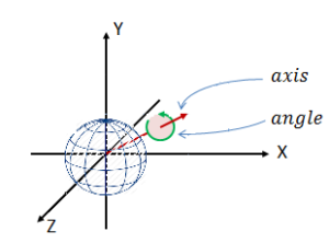
In the hands of others, notably Issai Schur, Élie Cartan, and Hermann Weyl, the notion of representation was extended to continuous groups, the most important example being the group of rotations about a given point in three-dimensional space. This group has dimension three. For example, if we are thinking of rotations of the Earth about its center, we have to first decide what point we shall rotate the north pole about. To describe this point takes two coordinates. We have then to add a third because we are still free to rotate around the new pole through an angle, whose size can be between 0^\circ and 360^\circ . It is the representations of this group to which the oracular pronouncement of Hermann Weyl about quantum numbers and group representations applies.
The understanding of the fundamental role of this group and its representations in atomic spectroscopy and, ultimately, not only of representations of this group but also of many other groups as well in various domains of quantum physics led to a vigorous interest of the representation theory of finite and of continuous groups on the part of both physicists and mathematicians. The mathematical development remained for some time largely independent of the questions raised by spectroscopy and the later, more sophisticated theories of fundamental particles. There is not even, so far as I can see, a close relation between Weyl’s reflections on group theory and quantum mechanics and his fundamental contributions to the mathematics of group representations. Before describing how the concepts introduced by the physicists found their way back into mathematics, I recall briefly the issues that faced spectroscopists in the period after 1885, when the structure of the frequencies or wavelengths–-thus the colour in so far as the light is visible and not in the infrared or ultraviolet regime–-of the light emitted by hydrogen atoms was examined by Balmer, and in the period after 1913, when N. Bohr introduced his first quantum-mechanical explanations.
There are at least two physical issues to keep in mind when reconstructing the path that leads from the ideas of Dedekind, Kronecker and Frobenius through spectroscopy to the introduction of continuous groups and their representations into the theory of automorphic forms. The first has nothing to do with groups. The frequencies emitted by, say, the hydrogen atom are not arbitrary. There will be intervals of frequencies, in principle infinite in length, that can all be emitted, but these continuous intervals do not concern us at the moment. What concerns us are the frequencies that appear in isolation from the others. The Balmer formula recognizes, as do other formulas of the same nature, that it is best to express them as a difference. Bohr recognized that this difference should be taken seriously as a difference of energies, the energies of the atomic states that preceded and followed the emission of light, this being the energy of the emitted photon.
In the network of rectangles in Diagram A, I have left no place for linear algebra, which provides in the contemporary world the material for a mathematical course perhaps even more basic than calculus. It is in the context of linear algebra that the possible energies are calculated, as proper values, characteristic values, or eigenvalues of matrices or linear operators. The notions of matrix or of linear operator are essentially the same. The other three terms, proper-, characteristic-, or eigen-values, refer to exactly the same notion and are all translations of the same word Eigenwerte. It is the last translation, barbaric as it is, that comes most easily to my tongue and to the tongue of most mathematicians. I explain the notion with the help of the two simultaneous linear equations:
\[\begin{eqnarray*}
4x+2y=\lambda x,
2x+y=\lambda y.
\end{eqnarray*}\]
For most values of \lambda, this equation has exactly one solution in (x, y), namely (0, 0), but for certain exceptional values of \lambda, at most two, it has an infinite number of solutions. These values of \lambda are called eigenvalues. They are calculated as the roots of
\[\begin{eqnarray*}
(\lambda-4)(\lambda-1)-2\cdot 2=\lambda^{2}-5\lambda=0.
\end{eqnarray*}\]
Here the matrix of coefficients is given by
\[\begin{pmatrix}
4 & 2 \\
2 & 1
\end{pmatrix}.\]
In general the four coefficients would be written as
\[\begin{pmatrix}
a & b \\
c & d
\end{pmatrix},\]
and the equation for \lambda would be
\[\begin{equation*}
(\lambda-a)(\lambda-d)-bc=0,
\end{equation*}\]
often written as
\[\begin{align}
\begin{vmatrix}
\lambda-a & -b\\
-c & \lambda-d
\end{vmatrix}=0.\tag{5.1}\end{align}\]
So it has two solutions. With a small effort of imagination, one can pass to equations with three, four, or an arbitrary number of unknowns, and therefore with three, four, or more eigenvalues. With even more imagination, one can generate an infinite number of eigenvalues by passing to infinite matrices or to linear operators on a space of infinite dimensions. This is done in mathematics and in quantum mechanics, where the equation (5.1) is closely related to Schrödinger’s equation
\[\begin{equation*}
i\hbar \dfrac{d}{dt}|\Psi(t)\rangle=\hat{H}|\Psi(t)\rangle,
\end{equation*}\]
and its eigenvalues are the energy levels. Here t denotes time, \hbar=h/2\pi is the reduced Planck constant, \hat{H} is the Hamiltonian and \Psi(t) is the state of the quantum system at time t. The above usually appears in both mathematics and quantum mechanics as a linear differential equation. There is some legerdemain here, but we are on solid ground, and if we are to understand Diagram A from top to bottom, it is essential to accept that, for the theory of algebraic numbers and for the theory of diophantine equations, group representations, even in their infinite-dimensional guise, have important insights to offer. They are for algebraic number theory, in which they arose, and for its practitioners, like the prodigal son, who had taken his journey into a far country, was lost, and is now found.
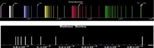
(Bottom) Balmer series governing discrete frequencies in the hydrogen emission spectrumWikimedia Commons
Although the appearance of infinitely many dimensions is troubling to those who, like the elder brother in the parable, served without transgression for so many years, they are, I believe, an inescapable element of any adequate theory. The linear operators came later than Bohr’s theory. Bohr’s calculation of the energy levels was inspired by simpler physical notions, but from the very beginning, these levels had to be infinite in number because the light was emitted with infinitely many different frequencies, the most interesting being those that occurred discretely. The initial theory was also, so far as I know, unencumbered by group representations. As a consequence, it could not fully explain the observed spectra.

The elements of the rotation group are given as acting on a three-dimensional space, the one with which we are familiar, it being clearly possible to compound one rotation r_{1} with a second r_{2} to obtain a third that is written as a product r_{2}r_{1}, thus defining the group law. So each rotation maps the space onto itself, but without destroying the straight lines. Each straight line is transformed into a second straight line. Such transformations are called linear. Although it is a little harder to imagine, many other groups can be realized as groups of linear transformations, and the same group can be realized in many different ways and in many different dimensions.
The frequencies appearing in the various series of frequencies, Lyman, Balmer, Paschen, or principal, sharp, diffuse, and so on, discovered by the spectroscopists in the closing decades of the nineteenth century and the first decades of the twentieth century, revealed themselves on closer and closer examination to have a structure whose complexities, among them the splitting of lines in the presence of a magnetic field, were only unravelled with an ingenuity and inventiveness that for an outsider almost pass belief. These complexities are all related either to the angular momenta of the particles–-nucleus or electrons–-involved and to their composition, in which to complicate matters the exclusion principle of Pauli has major effects. The key to the analysis of the angular momenta is the rotation group and its different representations. The exclusion principle of Pauli is expressed by a much simpler group, one with only two elements, or, perhaps more precisely, by the group of all permutations. It is not our purpose here to attempt to follow the physicists in their ruminations except to conclude that the energy levels that are calculated mathematically have a structure that is very difficult to analyze, in part for dynamical reasons–-thus in part expressed by a differential equation–-and in part because of the mathematical complexities that arise when several representations of the group of rotations appear simultaneously. There are marvelous early texts on spectroscopy for the more adventurous to consult.
The exclusion principle of Pauli is expressed by the group of all permutations.
As the theory developed and as relativity theory made its appearance in quantum mechanics, so that the group of rotations was to some extent displaced by the Lorentz group, it was suggested by two physicists, separately and independently although they were brothers-in-law, Paul Dirac and Eugene Wigner, that the representations of the Lorentz group, of which the basic ones–-the technical term is “irreducible”–-those from which the others can be constructed with the help of familiar mathematical methods, would be the most important, could be of some physical interest. In contrast to the group of rotations, for which a fixed centre is demanded, the possibility of motion is implicit in the Lorentz group, so that not only the complex structure entailed by the simultaneous appearance of several representations of the rotation group but also the mixture of discrete and continuous spectra met in spectroscopy and given through the Schrödinger equation or Heisenberg matrix appear and are to be analyzed together. This entails representations in an infinite number of dimensions. The physical interest never, so far as I know, materialized. Nevertheless a former student of Dirac, Harish-Chandra, whose thesis was inspired by the suggestion of Dirac and Wigner and who, having turned to mathematics, very quickly returned to the suggestion, his reflections now informed by a mathematical perspective, created over the years a magnificent and absolutely general mathematical theory. It is, to a considerable extent–-although there are other factors–-this theory that enlarges the optic of class field theory and allows it to encompass, at least potentially, not merely the very limited, but nonetheless extremely difficult, class of equations in one variable with which it began but, as in the lowest rectangle on the left of Diagram A, all the diophantine equations of modern algebraic geometry.
What is fascinating here is not how much or how little the content of the rectangle automorphic forms is influenced by the theory of infinite-dimensional representations rather than by algebraic number theory or by, say, the theory of elliptic modular forms, but rather the curious journey of representation theory, arising in the elementary calculations of Dedekind of group determinants and the elegant and astonishing theory to which they led Frobenius, and then passing through the far countries of quantum mechanics and relativity theory. I would not suggest that it there wasted its substance–-on the contrary, in spite of this, not all have rejoiced at its homecoming.
Scenic as the route from algebraic numbers and ideals to automorphic forms and functoriality over quantum theory and relativity is, and essential as the concepts acquired on traversing it are, the core of the matter seems to me to lie rather in the little understood triangular region formed by Euler products, class field theory and automorphic forms. Frankness demands that something be said about it, but the explanations will have no meaning for those readers with little mathematical training, and almost none for most mathematicians. It would, nevertheless, be irresponsible to omit them entirely and not to confess that something very important is lacking in my explanations. I postpone them to the final section.
Cartesian Geometry and the Mysteries of Integration
We spent a good deal of time in §1 (“From Then to Now”),2 recalling, largely for the benefit of those who may not have seen them before, the basic formulas for the integration of rational functions and their relation to the fundamental theorem of algebra.
Although this theorem was certainly not known to Descartes, it is difficult not to recall it when reading the essay on geometry that supplements his Discours de la méthode. Much of his essay is given over to matters every bit as technical as those to which we have introduced the reader in the preceding passages, but in the initial pages it is his enthusiasm about some simple structural elements that appear when coordinates are introduced into planar geometry, especially about the degree of a curve and the influence of degree on the properties of intersection, that is most in evidence. The influence of Apollonius is transparent.
Consider in the plane a curve of the form
\[\begin{equation}
y=a_{n}x^{n}+a_{n−1}x^{n−1}+\cdots+a_{1}x+a_{0},\tag{6.1}
\end{equation}\]
supposing at first that a_{n} \neq 0. The number of intersections of this curve with the line y= b is the number of roots of
\[\begin{equation*}
X^{n}+\frac{a_{n-1}}{a_{n}}X^{n-1}+\cdots +\frac{a_{1}}{a_{n}}X+\frac{a_{0}-b}{a_{n}}=0,
\end{equation*}\]
a root \theta leading to the intersection (\theta, b). If we, to take care of accidental degeneracy, count a multiple root as a multiple intersection and if we, in addition, include complex roots of the equation as complex intersections, then the line and the curve always intersect in exactly n points. Thus the geometric form of the solutions of the simultaneous equations,
\[\begin{equation*}
y=b, \quad y=a_{n}x^{n}+a_{n-1}x^{n-1}+\cdots + a_{1}x+a_{0},
\end{equation*}\]
is determined by the algebraic form. An intersection of a curve of degree one, the line y= b, and a curve of degree n, the curve (6.1), is a collection with 1 \times n points. Its geometric form is determined by the algebraic form of the simultaneous equations. This is a simple example of the principle of Descartes.
There is another modern feature that is not explicit in the essay. A line is of degree one, so that two lines have 1 \times 1 = 1 points of intersection. This is, of course, not so if there the lines are parallel. As a remedy, one adds to the plane a line at infinity and obtains the projective plane in which a curve of degree m and a curve of degree n have exactly mn intersections, counted of course with multiplicities to take points at which the curves become tangent into account. The most familiar examples arise in the theory of conic sections, in which many of the intersections are complex, so that they do not appear in the usual diagrams. An ellipse and a circle can have four points of intersection, but if the ellipse becomes a circle, these points all become complex. If the circles coincide, there is a degeneracy about which nothing can be done and there is no question of counting points.
That the algebra contains the geometry, expressed so simply and intuitively, by the assertion that the number of intersections of two curves of degrees m and n is mn, manifests itself in very sophisticated ways in modern geometry and number theory and is the theme of the column on the left in the diagrams. To see this, we recall the geometry of plane curves, but for which we allow not just real but also complex points. Start with the line, thus a single coordinate z, but now complex so that z = x + iy, x and y real. Thus the line becomes a plane. To the line has to be added a point at infinity to form the projective line. It is a single point, but the effect is to take the infinite plane of possible z and to fold it into a pouch that is closed at the top to form a ball, at first shapeless but that it is best to think of as spherical. This is a step that, although elementary and intuitive, requires some experience, some explanations, and some diagrams to grasp. It has many consequences as do the other improvements of Descartes’s intuitions.
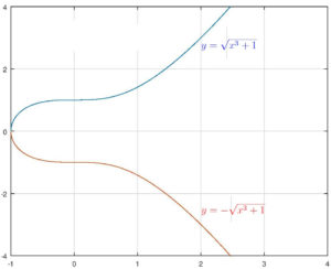
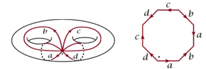
Consider the curve E~:~y^2=x^3+1, one of those that so fascinated Jacobi. If we plot it in the usual way, there appears to be nothing of great interest in it. It extends smoothly from the left to the right of the page, rising steadily, y\geq 0, or falling, y\leq 0. With the projective plane in mind, we observe that the tangents have a slope whose magnitude increases to \infty as we move to the left or to the right. So they become parallel and their point of intersection moves off to infinity. Thus, in the context of projective geometry, there is at least one additional point to be added to the curve, the common point of intersection of two lines parallel to the vertical axis of ordinates. This is a point on the line at infinity in the projective plane. So the curve E, or at least the points on it with real coordinates, has to be completed and the result is a closed loop. The two infinite ends close on each other. This done, there are still points with complex coordinates. It is more of an effort to envisage them. As x sweeps out over the imaginary plane, it is completed by assigning two different values for y, namely y=\pm\sqrt{x^3+1}. This yields a surface which it is an art, one introduced, I believe, by Riemann, to visualize. The surface is that of a ring or, if one likes, a doughnut, on which the curve of real points is a closed curve, say a meridian. On such a surface, there are many other closed curves, of which the latitudinal curves are the first to suggest themselves.
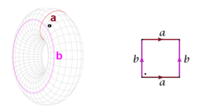
Notice that if we take a doughnut-shaped surface, say an inner-tube,3 and cut it first along a meridian and then along a latitudinal curve, the result can be unrolled as a rectangular sheet, so that these two curves, or at least the number 2, is a significant element of the geometry, or better, topology of the surface.4 Can this topology be seen directly in its algebraic form? It can, and not just for plane curves but for curves, surfaces, and higher-dimensional varieties in the plane, in three-dimensional projective space, or in coordinate space of any dimension. So the fundamental theorem of algebra has unsuspected implications. Basically, all of the geometry of the variety–-the mathematical term for curve, surface, three-fold, and so on–-of complex points defined by algebraic equations can be recovered in a prescriptive manner from the equations themselves. The simplest cases are, as already observed, the number of points on the locus in the projective plane defined by two equations or in three-dimensional projective space by three.
For curves in the plane, this is best expressed by a theorem attributed in its general form to Niels Abel, a Norwegian mathematician who died young in 1829. It is a theorem about integrals, but as one learns in introductory calculus and as is clear from §1 (“From Then to Now”), integration is for many purposes an entirely algebraic matter. We continue to examine the curve E. We consider integrals of the form
\[\begin{eqnarray*}
\int F(x,y)dx,
\end{eqnarray*}\]
in which it is understood that y=\sqrt{x^3+1} depends on x and that F is a quotient of two polynomials in x and y. A typical example is (1.6), which is
\[\begin{eqnarray*}
\int\dfrac{dx}{y}.
\end{eqnarray*}\]
Many of the integrals will contain a logarithmic term as do some of the integrals in (1.1).5 It is easy to see how. The logarithm is not an algebraic function and it is best to exclude these integrals from the statement of Abel’s theorem. They would only add to its complexity.
If we add to F a function that is a derivative, thus a function of the form dG/dx, where G is also a quotient of two polynomials in x and y, and if F_1=F+dG/dx, then
\[\begin{eqnarray*}
\int F_1(x,y)dx=\int F(x,y)\,dx+G(x,y),
\end{eqnarray*}\]
so that from the point of view of integration theory, one of these functions is tantamount to the other, or at least just as easily treated. So we need to study the integrals only for representatives of the possible functions F up to such modifications.
Up to such modifications the pertinent F can all be written in the form
\[\begin{equation}\label{6.2}
\dfrac{A}{y}+\dfrac{Bx}{y},
\tag{6.2}
\end{equation}\]
where A and B are two constants. To show this requires a little calculation but it is not difficult. It shows that the number 2, significant for the topology, also appears in the algebra. Of course, one example is not convincing, but, according to Abel’s theorem, the same principles govern all curves, and according to subsequent developments, algebraic varieties of any dimension. For example, the surface given by y^2=x^6-1 is a double doughnut, thus a little like a pretzel, the number of curves along which it must be cut before it can be developed onto the plane is four, and (6.2) is replaced by
\[\begin{equation}
\dfrac{A}{y}+\dfrac{Bx}{y}+\dfrac{Cx^2}{y}+\dfrac{Dx^3}{y}.\tag{6.3}
\label{6.3}
\end{equation}\]
By the way, for the curve given by the complex projective line itself, thus with a single parameter x, the associated surface is a sphere. So there are no closed curves on it that cannot be deformed continuously to a point and the two basic integrands of (6.2) or the four of (6.3) are not necessary at all. Every integral is given by a rational function. This corresponds to the second equation of (1.3)
\[\int\frac{1}{(x-a)^n}dx=-\frac{1}{n-1} \frac{1}{(x-a)^{n-1}},\quad n>1\]
and, one would wish, to the experience of every student beginning the study of the calculus.
This intimate relation between the study of algebraic equations and topology has, as already mentioned, even more surprising expressions suggested–-or conjectured–-about sixty years ago by André Weil, realized by Alexander Grothendieck, and now central to the thinking of many specialists of the theory of numbers. They appear at the bottom of the column on the left of Diagram A: contemporary algebraic geometry, diophantine equations, motives, \ell-adic representations. They are therefore central to the goals of the theories that contemporary pure mathematicians are trying to construct.
If the equations under considerations have, say, coefficients that are rational numbers, as does, say, the equation y^2=x^3-1, then we can consider the solutions that are algebraic numbers. This brings Galois theory and Galois groups into play. Indeed the number of arbitrary coefficients that appear in (6.2) or (6.3) is, in fact, a dimension and this is so both from an algebraic standpoint and from a topological standpoint. The theory of Weil–Grothendieck–-to which of course others have made important contributions–-reveals that these dimensions are also the dimensions of the representations of the Galois group. The representations are not of the same nature as those appearing in spectroscopy or in the theory of automorphic forms as in §5 (“From Algebraic Number Theory to Spectroscopy”), but very similar.
This intimate relation between the study of algebraic equations and topology has even more surprising expressions.
As an apparently simple, but still central and in the context of Diagram A, extremely difficult case, one can take the coefficients of equation (1.1) to be rational and consider it as a diophantine equation. Suppose the roots are distinct. They are algebraic numbers \theta_1,…,\theta_n and determine a field K, the collection of finite sums
\[\begin{eqnarray*}
\sum\limits_{n\geq 0}\alpha_{k_1,…,k_n}\theta_1^{k_1}\theta_2^{k_2}\cdots \theta_n^{k_n}.
\end{eqnarray*}\]
It is a Galois extension of the field k of rational numbers. If, for example, (1.1) is X^2+5=0, it is the field examined in §4 (“Algebraic Numbers During the Nineteenth Century”).6 The introduction of sophisticated theories of integration is no longer necessary. The algebraic equations do not determine a curve, a surface of anything so difficult; they determine a finite collection, the points \theta_1,…,\theta_n, and a group, the Galois group of K/k whose elements permute these points among themselves. The associated representation is defined directly and simply by these permutations.
In Recent Decades
A modern goal, of which I have been a proponent for many years, is not merely to extend the abelian class field theory described succinctly in §4 (“Algebraic Numbers During the Nineteenth Century”) to arbitrary Galois extensions K/k but to create a theory that contains it and relates more generally the representations produced by the Weil–Grothendieck principles to automorphic forms. The final result would be the theory envisaged in the final lines of Diagram A. After examining the materials so far available, I persuaded myself–-with reservations–-that the theory would develop in two stages, some elements of both being already available, first a correspondence for the representations for the varieties of dimension zero defined by equations like (1.1), and then a second stage, the passage to varieties of any dimension. Although the second stage is implicit in the diagram, there are some aspects of it, probably the critical ones, with which I have not been particularly engaged and about which I have nothing to say here. I have as much familiarity as anyone with the first stage, but to describe it in any detail would be an imposition even on the most dedicated reader and somewhat presumptuous as well, because with it we enter a region in which the intimations that I described earlier play a large part. Even though there is a great deal left to be done, a few words may do no harm.
The arguments for the first stage can, in my view, which is not universally shared, be formulated entirely in the context of the theory of automorphic forms without any reference to geometry, as a part of what I call functoriality. This will not be an easy matter, but we have, I believe, begun. As was observed at the end of §4 (“Algebraic Numbers During the Nineteenth Century”), class field theory in its classical form, rested on two considerations: a careful study of Galois extensions K/k of a very specific type with, in particular, abelian Galois groups; the study of the decomposition of prime ideals in k in the larger field K. Similar features may very well appear in the proof of functoriality. First of all, a similar study of Galois extensions but with arbitrary Galois groups, perhaps, as for the abelian case, with certain simplifying assumptions; no one has yet undertaken this, perhaps simply because it offered until now no rewards.
The general form of the study of the decomposition of prime ideals is impossible to describe within a brief compass. The current theory of automorphic forms requires the introduction of groups that, like those appearing in the suggestion of Dirac–Wigner, admit infinite-dimensional representations, but at the same time are related not directly to the decomposition of prime ideals as such but to the decomposition of matrices with elements from these prime ideals and their powers. The necessary theorems or propositions are much more complex and have a much larger component of techniques from the integral and differential calculus and its successor, modern analysis. A beginning on their development is made in the paper “La formule des traces et fonctorialit\’e: le d\’ebut d’un programme”, written in collaboration with Ngô Bao Châu and Edward Frenkel.
I have suggested elsewhere that functoriality once acquired, the passage from motives to automorphic forms with the help of p-adic deformations, a standard technique, exploited in particular by Andrew Wiles, will become a much more effective and much less haphazard procedure than at present. \blacksquare
Footnotes
- “What the farmer does not know, he does not eat either.”. ↩
- See Part 1 of this article: Robert P. Langlands. “Is There Beauty in Mathematical Theories? (Part 1). Bhāvanā. Jan 2019. 3(1). ↩
- The Torus \mathbb{T}^2 ↩
- This is the number of curves required, cutting along which the surface transforms to a polygon in the plane; for the double torus or the genus two surface, the number of such curves is four, resulting in the polygon to be an octagon. ↩
- X^n+a_{n-1}X^{n-1}+\cdots+a_1X+a_0=0. ↩
- See Part 2 of this article: Robert P. Langlands. “Is There Beauty in Mathematical Theories? (Part 2). Bhāvanā. Apr 2019. 3(2). ↩