In this part, we shall discuss three topics from the mathematics of the Vedic and Sūtra periods. First, the mathematical significance of the number-vocabulary in the Vedic treatises. This necessitates a discussion on the distinction between the verbal decimal nomenclature and the decimal place-value notation and the connection between the two. The focus will be on decimal nomenclature and decimal expansion; the history of the decimal notation in India (as distinct from decimal nomenclature) will be discussed in the next part. However, references to the decimal notation will be frequently made for clarity through comparative discussions.
Second, we give examples of the knowledge of fundamental arithmetic operations, often involving large numbers, that occasionally occur in Vedic and Sūtra literature in a matter-of-fact way. Precise methods are described only in later post-Vedic treatises and no explicit mention of the methods employed during the Vedic period are available. We shall give examples of the explicit Indian methods for performing fundamental operations in the next part of the series.
Third, we discuss the brilliant enumerative or combinatorial ideas in Chapter 8 of the prosody text Chandaḥ-sūtra of Piṅgalācārya. Just as the Śulba-sūtras present the mathematical knowledge required in the constructions of the Vedic fire-altars, a major portion of the last chapter of the Chandaḥ-sūtra addresses mathematical questions arising from an analysis of metres (chandas). Thus, Piṅgala’s mathematical gems were mere incidental offshoots of the study of metres which had deep spiritual significance in the Vedic tradition. To illustrate the mathematical impact of Piṅgalācārya’s treatise, we shall also present a few examples of important mathematical results from post-Vedic texts which are inspired by, and are natural extensions of, his mathematical innovations.
The decimal system in Vedic literature
In this section, we shall highlight the decimal number-vocabulary in the Vedas, indicate its pivotal role in the evolution of the decimal notation and discuss its mathematical sophistication. We shall particularly highlight the seminal role of decimal expansion, the basis of the Vedic number-vocabulary, in the evolution of fundamental ideas of algebraic mathematics.
Decimal notation and decimal nomenclature
The word “decimal” (“pertaining to ten”) is derived from the Latin decimalis (adjective for “ten”) and decem (ten), resembling the Sanskrit daśama (tenth) and daśan (ten).
For clarity, we make a distinction between the two main familiar forms of the decimal system of representing numbers:
- decimal place-value notation (decimal notation, in short), e.g., “2019”.
- (verbal) decimal nomenclature, e.g., “two thousand and nineteen”.
They are convenient for written and oral communications respectively.
The only ingredients for our standard decimal notation are ten distinct symbols called “digits” – one each for the nine primary numbers (1,2,3,4,5,6,7,8,9) and an additional tenth symbol “0” which is used to denote the absence of any of these nine digits at a requisite place of some number (e.g., in 2019, the symbol 0 is used to denote the absence of any of the nine primary numbers in the hundred’s place in the number “two thousand and nineteen”).
Every number, no matter how large, is expressed through these ten figures using the “place-value” (or “positional value”) principle by which a digit d in the rth position (place) from the right is imparted the place-value d \times 10^{r-1}. For instance, in the number denoted by 2019 in decimal notation, the digit 2 (situated in the fourth place from the right) acquires the value “two thousand (2 \times 10^3)”. The Sanskrit word for “digit” is aṅka (literally, “mark”) and the term for “place” is sthāna.
In our standard verbal decimal nomenclature, each number is expressed through nine words (“one”, “two”, … ,“nine” in English) and number-names for the “powers of ten” (like “hundred”, “thousand”, etc.). Here the number-names for the powers 10^n play the role of the place-value principle. The concept of zero as a place-holder is not required for the verbal expression of a number. For convenience, some additional derived words are adopted (like “eleven” for “one and ten”, …, “nineteen” for “nine and ten”, “twenty” for “two ten”, etc). In the orally transmitted Vedic literature, we see this verbal form of the decimal system (not the decimal notation).
Both the above forms originated, and were developed in India; the decimal notation evolved within the early centuries of the Common Era, while the verbal decimal nomenclature was already in vogue when the Ṛgveda, the most ancient extant world literature, was compiled. In addition, there was another system in India of expressing numbers (both orally and in writing) using place-value in place of number-names for powers of ten but using words in place of digits; the words were usually arranged in ascending powers of ten; like 2107 being expressed as “seven-zero-one-two”. This system suited the tradition of oral transmission. The term “numeral” is usually used as a synonym for a “digit” but is sometimes also used for the word-name (“one”, “two”, etc.) of a digit.
Decimal expansion
At the heart of both the Vedic decimal nomenclature and the decimal notation lies the mathematical principle that every natural number N can be expressed as a “decimal expansion”
\[\begin{equation}\label{decimalexpansion}
N=10^na_n+ \cdots + 100a_2+ 10a_1 + a_0,
\end{equation}\]where a_0, a_1, …, a_n are numbers between 0 and 9. It is a polynomial-like expansion with x being replaced by 10. The connection between the two expansions will be discussed in subsequent subsections.
As the Vedic number-names are evidently older than the perfected decimal notation, the genesis of this great idea of “decimal expansion” of numbers has to be traced to the unknown creators of the Vedic number-vocabulary. However, though expositions on the history of mathematics generally shower high praise on the decimal notation and the zero, they tend to overlook the enormous significance of the verbal form of the decimal system, especially its aspect of decimal expansion (1).
The decimal expansion involves recursive (repeated) applications of the algebraic principle of “division with remainder” which states that for any pair of natural numbers a and b, a=qb+rfor some numbers q,r with 0 \le r < b.
As an illustration, note that the decimal expansion of 2019 can be obtained by applying the above principle thrice, starting with a=2019 and b=10:
\[\begin{align*}
2019& = 201 \times 10+9\\
&=(20 \times 10+1) \times 10 +9\\
&=20 \times 10^2+1 \times 10+9 \\
&=(2 \times 10) \times 10^2+1 \times 10+9 \\
&=2 \times 10^3+ 1 \times 10+9.
\end{align*}\]The principle of “division with remainder” is an important principle that pervades much of the later Greek, Indian and modern mathematics. For instance, it is crucially involved in the following algorithms which were known in India by the time of Āryabhaṭa (499 CE):
- Long division; extraction of square root and cube root.
- Finding the GCD d of a,b (which also occurs in Euclid’s Elements).
- Finding integers x,y such that d=ax-by.
The theoretical principle of “division with remainder” is often called the “Division Algorithm”. The terminology is misleading. For, the so-called “Division Algorithm” is an existential statement and, by itself, does not describe a practical algorithm to compute q and r quickly when a and b are large numbers and q,r cannot be readily seen by inspection.
To better appreciate the algebraic nature of the decimal expansion of numbers, we first recall the concept of a “polynomial”.
Polynomials: A brief introduction
Recall that an expression like a_0+a_1x+\cdots+a_nx^n is called a polynomial in one indeterminate (or variable) x with coefficients a_0, …, a_n, while an expression like a_0+a_1x+\cdots+a_nx^n+\cdots with possibly infinitely many terms, is called a power series. Polynomials and power series are as basic to modern mathematics as numbers. One can add, subtract and multiply two polynomials (respectively, power series) to obtain another polynomial (respectively, power series). As we shall see later, the arithmetic of numbers based on their decimal expansions influenced the algebra of polynomials. The close analogy between numbers and polynomials is not quite an accident.
“Classical Algebra” refers primarily to the study of polynomials: the roots (or solutions) of polynomial equations, the relationships between roots and coefficients, etc. While “polynomials” formed the cornerstone of Classical Algebra, they remain the central objects of study in Modern Algebra and Algebraic Geometry—sometimes explicitly and sometimes through disguises like “field extensions” or “algebraic varieties”.
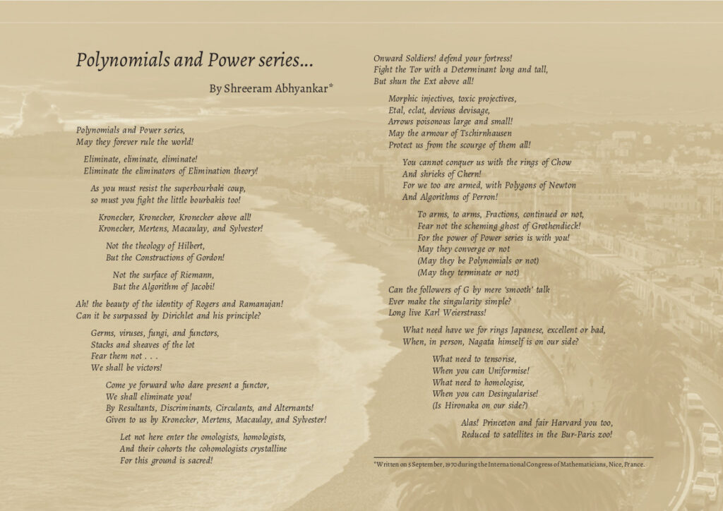
The mathematical poem titled “Polynomials and Power Series” by the eminent mathematician S.S.Abhyankar (1930–2012) begins with the exaltation1.:
May they forever rule the world.
A general polynomial of degree n in one variable may be represented in the following two ways (with a_n \ne 0):
- a_nx^n+a_{n-1}x^{n-1}+\cdots+a_2x^2+a_1x+a_0.
- (a_n, a_{n-1}, …, a_2, a_1, a_0).
For instance, the polynomial usually represented as 2x^3+ x +9 (i.e., in the form (i)) will be denoted by (2,0,1,9) in form (ii).
While expression (i) is the commonly used form for a polynomial, the sequence (ii) is often used in Abstract Algebra to formally define a polynomial. We note two contrasting features of these two representations.
First, the variable x is displayed in the more familiar form (i), but suppressed in form (ii).
Second, in form (i), we need not write a coefficient if it is zero (e.g., the coefficient of x^2 is not written in 2x^3+x+9); but in form (ii), 0 has to be put as an entry when any coefficient is zero.
Are we not reminded of the analogous representations of numbers in the decimal system in two ways (verbal and symbolic):
- Two thousand One ten and Nine (Two thousand and nineteen)
- 2019
Two thousand One ten & Nine
\[\begin{array}{lll}
&\leftrightarrow & 2x^3{\rm ~}+x+9 \\
{\rm~~~~~~~~~~~~~~~~~}2{\rm ~~~~} 0 {\rm ~~~~}1 {\rm ~~~~} 9 & \leftrightarrow &(2,~~~0,~~~1,~~~9)
\end{array}\]Before discussing the correspondence between Vedic number-vocabulary and usual polynomial representation (i), we first mention the salient features of the Vedic number-vocabulary.
Decimal number-vocabulary in Ṛgveda
The verbal form of the decimal system was already in vogue when the Ṛgveda, the oldest Veda and the oldest extant body of world literature, was compiled. The Ṛgveda has single-word terms for
- the nine primary numbers:
eka (1), dvi (2), tri (3), catur (4), pañca (5), ṣaṭ (6), sapta (7), aṣṭa (8) and nava (9); - the first nine multiples of ten:
daśa (10), viṁśati (20), triṁśat (30), catvāriṁ śat (40), pañcāśat (50), ṣaṣṭi (60), saptati (70), aśīti (80) and navati (90); and - the first four powers of ten: daśa (10), śata (10^2), sahasra (10^3) and ayuta (10^4).
The above terms are suitably combined, as in our present verbal decimal terminology, to name other numbers. For instance, the number “seven hundred and twenty” is expressed in Ṛgveda (1.164.11) as sapta śatāni viṁśatiḥ.
Numbers are represented in the decimal system in the Ṛgveda, in all other Vedic treatises, and all subsequent Indian texts. No other base occurs in ancient Indian literature, except for a few instances of base 100.
Regarding the etymology of daśa (ten), the ancient lexicographer Yāska (6th century BCE or earlier) says:
i.e., daśa is so called as it closes off a sequence of numbers (1, 2, 3, …) and as its effect can be seen (in forming the next sequence). It may be recalled that similar-sounding Vedic words das, dasma, dasra have the sense of completing, fulfilling, accomplishing; das also has the related sense of getting exhausted. Yāska says that śata (hundred) derives from daśadaśa (ten ten’s), without further explanation. We mention here that, due to their extreme antiquity, the etymology of Vedic words is often obscure; even ancient lexicographers had to use ingenious guesses, rather than definitive knowledge.
In the Vedic culture, a special mystic significance had been attached to the powers hundred, thousand and ten thousand. The number hundred represents a general fullness. Ten layers of hundred symbolizes an entire plenitude, an absolute completeness, and a word for plentiful—sahasra, was adopted for it. The word sahasra is derived from the root sahas which stands for “mighty”, “powerful”, “victorious”, “strength”, “force”, etc.; thus, sahasra is mighty, a huge number. Ten thousand too is special as the mystics saw in the illumined mind ten subtle powers, each having an entire plenitude ([1], pp. 301–302, 4162), and a word conveying a sense of abundance—ayuta (unbounded), was adopted for it. The Sanskrit meanings of yuta include “attached”, “fastened”, “joined”, “connected”, “united”, “combined”. (Hence, yuta is also the Sanskrit word for “addition” in arithmetic.) The negation ayuta means “unjoined”, “not yoked”, “unbounded”, etc.
 |
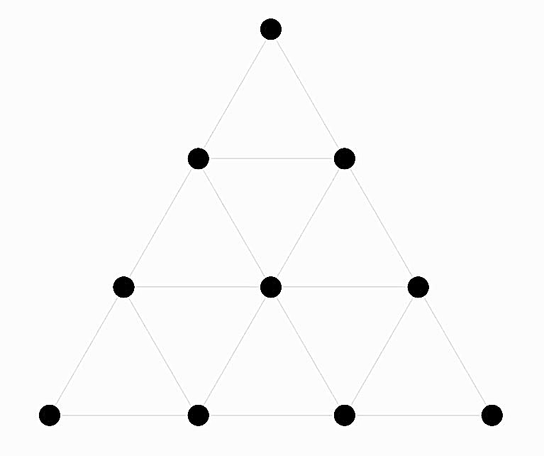 |
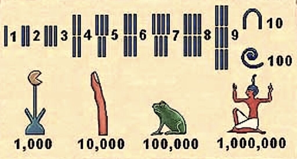
One may then surmise that the choice of base ten and the coining of number-names for certain powers of ten might have a mystic genesis (see [12] for details). The mystic civilisation of ancient Egypt also used base ten and had special pictorial symbols, with possible allegorical connotations, for powers of ten up to 10^7 (ten million). However, the Egyptian system of hieroglyphs did not anticipate the idea of “place-value”, or any analogue. The Pythagoreans, inheritors of Egyptian and other mystic traditions, considered ten to be a perfect number (reminiscent of the completeness of das). They considered as sacred the tetractys, the triangular figure with ten special points arranged symmetrically in four rows containing one, two, three and four points (1+2+3+4=10), representing, among other things, the dimensions zero (point), one (line defined by two points), two (plane/triangle defined by three points) and three (tetrahedron defined by four points) respectively.
Medhātithi’s list for powers of ten
An enunciation of the concept of “powers of ten” can be seen in the following verse of Medhātithi in Vājasaneyī Saṁhitā (17.2) of the Śukla Yajurveda, where numbers are being increased by taking progressively higher powers of ten:
cāyutaṁ cāyutaṁ ca niyutaṁ ca niyutaṁ ca prayutaṁ cārbudaṁ ca nyarbudaṁ ca samudraś
ca madhyaṁ cāntaśca parārdhaścaitā me’ agna’ iṣṭakā dhenavaḥ santvamutrāmuṣmilloke
A literal translation would be:
Here, Medhātithi explicitly records single-word terms for progressively higher powers of ten up to one billion (10^{12}): eka (1), daśa (10), śata (10^2), sahasra (10^3), ayuta (10^4), niyuta (10^5), prayuta (10^6), arbuda (10^7), nyarbuda (10^8), samudra (10^9), madhya (10^{10}), anta (10^{11}), parārdha (10^{12}). Moreover, each of these terms is perceived, and practically defined, to be 10 times the preceding term.
We see that words charged with the sense of the extraordinary, of the surpassing of usual frontiers, being adopted as specific terms for high powers of ten: a word for the vast ocean (samudra), a word for the ultimate limit (anta) and finally the word for the luminous upper half of existence (parārdha) beyond the ordinary firmaments of our consciousness.
Large powers of ten in other very ancient Indian texts
Medhātithi’s terms occur with some variations, sometimes with further extensions, in other Saṁhitā and Brāhmaṇa texts. Terms for much higher powers of ten are mentioned in subsequent literature. An anonymous Jaina work Amalasiddhi has terms for all powers of ten up to 10^{96} (daśa-ananta). A Pali grammar treatise of Kāccāyana lists number-names up to 10^{140}, named asaṅkhyeya.
When convenient, centesimal (multiples of 100) scales have been used in India for expressing numbers larger than thousand. The Ṛgveda (1.53.9) describes 60099 as ṣaṣṭiṁ sahasrā navatiṁnava (sixty thousands ninetynine); the Taittirīya Upaniṣad (2.8) adopts a centesimal scale to describe different orders of bliss and mentions Brahmānanda (the bliss of Brahman) to be 100^{10} times a unit of human bliss; there is a similar reference in the Bṛhadāraṇyaka Upaniṣad (4.3.33). In a dialogue in the Buddhist work Lalitavistara (c. 300 BCE), Lord Buddha lists numbers in multiples of 100 from koṭi (10^7) up to tallakṣaṇa (10^{53}). The Rāmāyaṇa uses a scale of hundred-thousand (10^5) to mention terms up to 10^{55} (mahaugha).
For expressing high powers of ten, Jaina and Buddhists texts use auxiliary bases like sahassa (thousand) and koṭi (ten million), resembling our English vocabulary; for instance, prayuta (10^{6}) would be dasasatasahassa (ten hundred thousand).
From Vedic number-names to the decimal notation
The decimal place-value notation is a pillar of modern civilization. Due to its simplicity, children all over the world can now learn basic arithmetic at an early age. This has been a major factor in the dissemination (almost a proletarianisation) of considerable scientific and technical knowledge, earlier restricted only to a gifted few. Mathematicians and historians have paid glowing tributes to this profound innovation. A.L.Basham remarks, “The unknown man who devised the new system was from the world’s point of view, after the Buddha, the most important son of India.” (see [2], pp. 495–496)
However, due to the exclusive focus on the decimal notation, it is often overlooked that a momentous step had been taken by the ancient Vedic seers (or their unknown predecessors) when they imparted single word-names to successive powers of ten, thereby sowing the seeds of the decimal “place-value” principle. In fact, these single-word terms are the verbal manifestations of the abstract place-value principle. For, the written decimal place-value notation is simply
- a suppression of the (place)-names for powers of ten from the verbal decimal expression of a number, along with
- the replacement of the single word-names for numerals “eka, …, nava” by digit-symbols (one symbol for one digit) and
- the use of a zero-symbol for the absent powers.
For instance, from the expression “two thousand nineteen” (i.e., “two thousand one ten and nine”),
- drop “thousand” and “ten”,
- replace “two” by “2”, “one” by “1” and “nine” by “9” and
- put a “0” (after “2”) to indicate that there is no “hundred” in the expression;
and we have the decimal place-value notation 2019.
All the three transitional steps are wonderful ideas, but one can see that the Vedic number-vocabulary had set the stage for the decimal notation. That the key to the decimal place value notation lies in the Vedic Sanskrit number-vocabulary had been pointed out by Swami Vivekananda in 1895 during a speech “India’s Gift to the World” delivered at the New York City (at the hall of the Long Island Historical Society, now renamed Brooklyn Historical Society). The report of his speech in the Brooklyn Standard Union, February 27, 1895, contains the following succinct remark (see [27], Vol. 2, p. 511):
Vedic number-vocabulary versus polynomials
We have been emphasizing a crucial aspect of the number-vocabulary of Vedic Sanskrit: assigning a single-word term for each power of ten, up to some large power. It is the presence of single-word terms that gives the number-vocabulary of Vedic Sanskrit a polynomial-like structure which enabled it to serve as a precursor to the written decimal notation with momentous mathematical consequences.
The Vedic Sanskrit system is unlike, say, the English terminology which is dependent on auxiliary bases like “thousand” and “million”. For instance, Vedic Sanskrit has a single-word term like anta instead of a complicated compound term like “hundred thousand million”.
The correspondence between Vedic number-vocabulary and the usual polynomial representation (i) is given by
- daśa (10) \leftrightarrow x,
- śata (10^2) \leftrightarrow x^2,
- sahasra (10^3) \leftrightarrow x^3,
- ayuta (10^4) \leftrightarrow x^4, etc.
It may appear that there is a difference between the polynomial representation and the Sanskrit number-vocabulary: unlike the symbols x^3, x^4, etc. (all derived from x), the names for the powers of ten are not derived from daśa (10). Here, one has to note the practical aspect of terminology: for oral communication, a distinct single-word term like “thousand” is much more convenient than a derived term like “ten-to-the-power-three”. Also, note that the apparent difference is peripheral to the issue. For, the passage of Medhātithi, quoted above, shows that each of the single-word terms for powers of ten was perceived, and practically defined, to be 10 times the preceding term. Indeed, the passage may be regarded as containing an enunciation of the concept of “powers of ten”.
To appreciate the merit of the Sanskrit system of having a single-word term for each power of ten (up to some large power), note that even the present English terminology of using auxiliary bases like “thousand” and “million” is less satisfactory for expressing very large numbers in words. This is effectively illustrated by G.Ifrah (see [18], pp. 428–429) by comparing the verbal representations of the number 523622198443682439 in English, Sanskrit and other systems.
The mathematical richness and sophistication of the Vedic verbal decimal system can be glimpsed from the fact that its invention would have required the realization and application of several abstract principles: the concept of powers of ten (a manifestation of the abstract place-value principle and the forerunner of the decimal place-value notation), the so-called division algorithm, recursive methods, and polynomial-like expansion.
From decimal expansion to the algebra of polynomials
A little reflection will show that the addition and multiplication of polynomials are analogous to the addition and multiplication in arithmetic based on the decimal system, except that some adjustment has to be made in arithmetic for “carrying over” due to the restriction that the numerals (corresponding to coefficients a_i) range from 0 to 9 only. One may also say that the simplicity of the standard arithmetical operations in the decimal system is due to the polynomial-like aspects of the system. An example will be cited in a later subsection.
This analogy between the arithmetic based on the decimal representation of numbers and the algebra of polynomials is no coincidence; the former indeed had influenced the latter. This comes out in the following passage from Isaac Newton, a pioneer in the study of polynomials and power series in modern Europe. Newton emphasizes that the arithmetic of decimal numbers provides a fruitful model for developing the arithmetic operations on algebraic expressions in variables. Recall that the Indian decimal system had become standard in Europe shortly before the arrival of Newton. Newton writes (1671):
The passage implicitly acknowledges that polynomials and power series are conscious extensions of the intrinsic algebraic ideas in the decimal system. The polynomial character of the decimal system partly explains why Indian stalwarts, who were used to the decimal system, could make rapid strides in “Algebra” – why Brahmagupta could describe the algebra of polynomials in several variables in the early seventh century or why Mādhavācārya (of Saṁgamagrāma) could describe the power series expansions of trigonometric functions in the fourteenth century (as we shall see in subsequent parts of this series).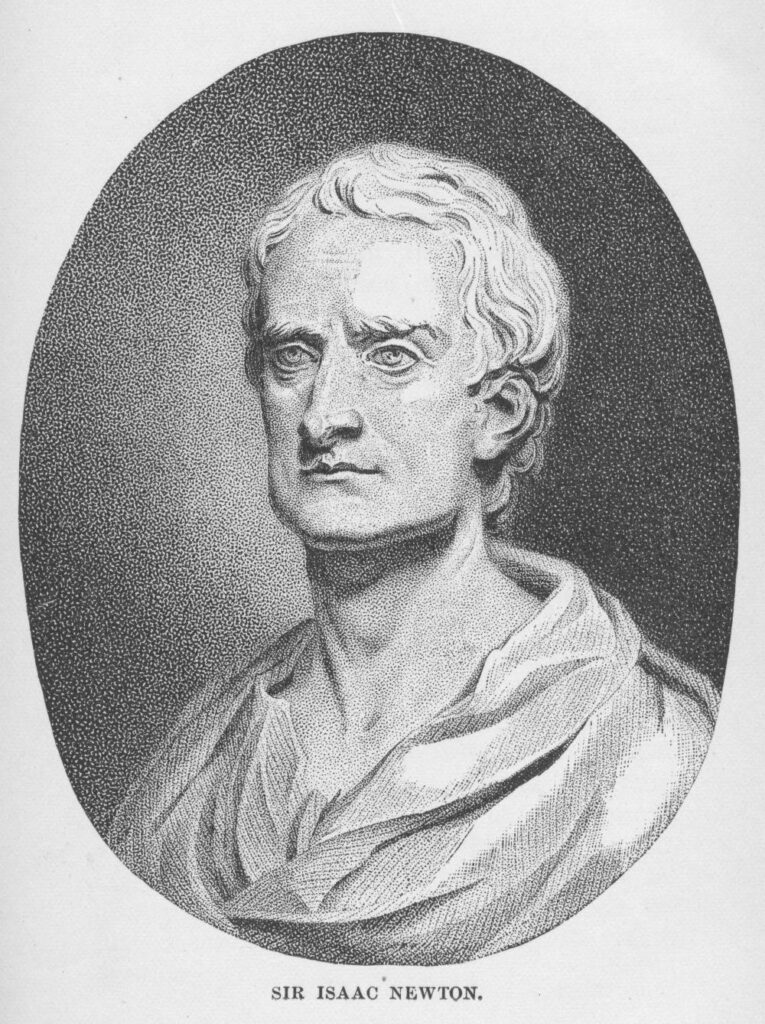
While Newton might have been referring to the decimal notation, his analogy applies to the Vedic verbal decimal system as well. In fact, as we have seen, this verbal decimal nomenclature is, in some sense, closer in spirit to the usual polynomial representation than even the decimal notation. This analogy should again give us an idea of the mathematical depth in the “Sanskrit words” forming the Vedic number representation.
The statement of Newton in 1671 shows that the algebra of polynomials and power series were conscious generalisations of arithmetic based on the decimal expansion of numbers. Since then, mathematicians have introduced other expansions for which the decimal expansion of numbers would have been a guiding model. Some of these expansions have become ubiquitous in modern mathematics. We now mention a few examples.
Decimal expansion as the model for the binary expansion
Analogous to the decimal expansion, every natural number N has the “binary expansion”
\[\begin{equation}\label{2adic}
N=2^na_n+ \cdots + 2a_1 + a_0,
\end{equation}\]where each a_i is either 0 or 1. As in decimal notation, the representation on the right is abbreviated as (a_n … a_0)_2 (or simply as a_n … a_0 when the base is understood); the consequent sequence of 0’s and 1’s is called a “binary number”. Thus, just as the decimal system expresses any number using only ten symbols, the “binary system” described above expresses any number using only two symbols 0 and 1. This binary system is at the heart of the modern computer and computer-based devices, since it enables a whole number to be represented as a string of binary switches: “on” (1) and “off” (0).
As a quick example, let us find the binary representation of 11 by the principle of division with remainder, making successive divisions by two:
\[\begin{align*}
11&=2 \times 5 +1\\
&=2 \times (2 \times 2+1)+1\\
&=2^3+2+1.
\end{align*}\]
We thus have
11=1 \times 2^3+0 \times 2^2+1 \times 2+1= (1011)_2In the notation of (\ref{2adic}), the binary digits of N from right to left a_0, a_1, …, a_n (here 1,1,0,1) can be quickly determined by the following general algorithm.
Set successively N_0:=N, N_1:=\frac{N_0-a_0}{2}=2^{n-1}a_n+ \cdots + a_1, N_2:=\frac{N_1-a_1}{2}=2^{n-2}a_n+ \cdots + a_2, and so on. The algorithm can then be described as follows.
- If N_0 is even, then a_0:=0; in this case, N_1=\frac{N_0}{2}. If N_0 is odd, then a_0:=1; in this case, N_1=\frac{N_0-1}{2}.
- Repeat the process with N_1 to obtain a_1, the next digit from the right, and N_2.
- Proceed likewise till all the digits of the binary representation are obtained:
If N_i is even, set a_i:=0 to obtain N_{i+1}=\frac{N_i}{2}If N_i is odd, set a_i:=1 to obtain N_{i+1}=\frac{N_i-1}{2}.
We indicate the rationale using, as an example, the binary representation of 11.
(i) In general, the last binary digit a_0 will be 0 or 1 depending on whether the number N_0 is even or odd. In our case, since 11 is odd, the last digit a_0 is 1.
(ii) Next, we consider N_0-a_0; here 11-1. The next binary digit from right a_1 will be 0 or 1 according as N_0-a_0 is divisible by 2^2 or not, i.e., according as N_1 is even or odd. In our example, N_1=5 is odd. So the penultimate digit a_1= 1.
(iii) Next, considering N_1-a_1 (here, 5-1), we see, as before, that the next binary digit a_2 will be 0 or 1 according as N_2 is even or odd. In our example, N_2=2 is even and hence a_2=0.
(iv) Likewise, the digit a_3 will be 0 or 1 according as N_3 is even or odd. In our example, N_3=1 is odd and hence a_3=1.
We describe below another method of obtaining the binary digits a_0, …, a_n, using similar ideas.
Exercise. With notation as before, set r_0:=N+1 and in general define r_{i+1} inductively by r_{i+1}=\frac{r_i}{2} if r_i is even and r_{i+1}=\frac{r_{i}+1}{2} if r_i is odd. For each i, 0 \le i \le n, define a sequence \{b_i\}_i as follows: b_i=1 if r_i is even and b_i=0 if r_i is odd. Show that, for each i, b_i=a_i.
Decimal expansion as the model for other expansions
For any prime p, one has the “p-adic expansion” of a natural number N as
N=a_np^n+ \cdots + a_1p + a_0, where each a_i lies between 0 to p-1. The system is extended by a mathematical process called “completion” (similar to the process of extending the set of polynomials to the set of power series). The numbers in the extended system are called “p-adic numbers”. They were introduced by Kurt Hensel in 1897. The p-adic numbers have powerful applications in modern number theory (including in the proof of Fermat’s Last Theorem by Andrew Wiles), analysis and algebra.
Even in the twentieth century, we find the celebrated algebraist S.S.Abhyankar acknowledging the idea of decimal expansion as a technical innovation in his own research. In his landmark “Kyoto paper”5 giving an exposition of the celebrated “Epimorphism Theorem”, Abhyankar writes about a crucial tool in the proof of the theorem:
Indeed, the title of Chapter 2 of the paper (Chapter 1 being “Introduction”) is “Decimal expansion” and that of Chapter 3 is “Polynomial expansion and approximate roots”, each of these two chapters comprising ten pages.
For a further appreciation of the mathematical significance of Vedic number-vocabulary, we shall henceforth discuss a few examples of the impact of the decimal expansion in the history of mathematics. Again, these discussions apply to both the verbal and the place-value notation forms of the decimal system.
Impact of decimal expansion: examples
The decimal system is largely responsible for the excellence attained by Indian mathematicians in arithmetic, astronomy and algebra. We give a few illustrations.
First, the polynomial-like decimal expansion of numbers is the basis for efficient methods of addition, subtraction, multiplication, division, and computing square roots and cube roots, which were developed in India at an early stage. We shall see several examples in the next part of this article. Below we discuss the standard multiplication algorithm which is a variant of an Indian algorithm that we will present in the next part.
The multiplication algorithm involves:
- the polynomial-like decimal expansion of whole numbers which is an algebraic concept;
- a realisation and skilful application of the “distributive property” of numbers (i.e., the rules a(b+c)=ab+ac and (a+b)c=ac+bc), an algebraic principle important enough to be conferred a distinct name; and
- adjustments for “carrying over”.
To see this, let us analyse the steps involved in the multiplication of 19 and 12.
First, the two numbers are partitioned by their respective decimal expansions:
19=1 \times 10 +9 {\rm ~~ and ~~} 12=1 \times 10+2. Then, making an efficient use of the distributive property, one performs separately
(1 \times 10 +9) \times 2 {\rm ~~ and ~~} (1 \times 10 +9) \times (1 \times 10), making use of decimal expansion all along; and then adds the products.
The two multiplications yield respectively:
2 \times 10 +10+8=3 \times 10+8 {\rm ~~ and ~~} 1 \times 100 + 9 \times 10; by adding the two products, we get
1 \times 100 +(3+9) \times 10+8 = 2 \times 100 +2 \times 10 +8 =228.
The above procedure presented in a tabular arrangement is shown below.
\[\begin{array}{lllllll}
&&~19& \longleftrightarrow& 1 \times 10 +9&& \\
&\times&~12& \longleftrightarrow& 1 \times 10+2&&\\
\hline
&&~38& \longleftrightarrow & (1 \times 10) \times 2 +9 \times 2&= & 2 \times 10 +10+8\\
&&190& \longleftrightarrow & (1 \times 10) \times (1 \times 10) + 9 \times (1 \times 10)&=& 1 \times 100 + 9 \times 10\\
\hline
&&228&\longleftrightarrow & 1 \times 100 + (3+9) \times 10+8&=& 1 \times 100 + 100+ 2 \times 10+8 \\
\hline
\end{array}\]Tabular arrangement of the multiplication operation (on the left) together with a step-by-step analysis (on the right).
Thus, the fluency in basic Arithmetic, in ancient India and modern Europe, is due to the decimal expansion.
Though the (polynomial-type) methods for performing arithmetical computations are described only in post-Vedic treatises, the polynomial aspect of the Vedic number-representation indicates that the Vedic computational methods too would have been akin to polynomial operations, using rules like (ten times ten is hundred), (ten times hundred is thousand), (hundred times hundred is ten-thousand) and so on, analogous to xx=x^2, xx^2=x^3, x^2x^2=x^4, etc.
Second, the decimal expansion has a dormant algebraic character which influenced the algebraic thinking of mathematicians in ancient India and modern Europe. We have seen that various expansions central to modern algebra and number theory, including polynomials and power series, are conscious generalizations of the decimal expansion of natural numbers. In India, Brahmagupta had defined the algebra of polynomials in 628 CE and Mādhavācārya had investigated the power series expansions of trigonometric functions in 14th century CE. Both the post-Vedic Indian geniuses had the advantage of being steeped in the decimal expansion gifted to them by the unknown seers of a remote past. As Newton would point out in 1671, a millennium after Brahmagupta, one can develop the operations (addition, multiplication, root extraction, etc.) with variables by imitating the methods of the arithmetic of the decimal system.
Third, the decimal expansion enabled Indians to express large numbers effortlessly, right from the Vedic Age. We mention two consequences.
Thanks to the decimal system, Indian astronomers could work with large time-frames, like cycles of 4320000 years, and thereby obtain strikingly accurate results. For instance, Āryabhaṭa (499 CE) estimated that the Earth rotates around its axis in 23 hours 56 minutes and 4.1 seconds, which matches the modern estimate (23 hours 56 minutes 4.09 seconds).
Again, it is due to the decimal system that Indian algebraists could venture into problems on equations whose solutions involve large numbers. One of the most glorious achievements of ancient Indian algebraists is their research on the problem of finding `integer’ solutions to linear and quadratic equations, a very important theme in modern number theory. Three of the greatest feats on the theme are:
- The kuṭṭaka (pulverization) method of Āryabhaṭa (499 CE) for finding positive integers x,y satisfying an equation ax-by=c, where a,b,c are known integers.
- A composition law of Brahmagupta (628 CE) on the solution space of the equation Dx^2+z=y^2, where D is a fixed number.
- The cakravāla method of Jayadeva (within the 11th century) for solving Dx^2+1=y^2 in integers, a celebrated problem of modern mathematics.
As an illustration of the kind of large numbers that get involved in the above problems, we mention that the smallest pair of integers satisfying 61x^2+1=y^2 is x=226153980, y=1766319049. And this example occurs in the Algebra treatise Bījagaṇita (1150 CE) of Bhāskarācārya. 500 years later, that is, soon after the decimal system got standardised in Europe, the equation Dx^2+1=y^2 (and the specific example 61x^2+1=y^2) would be highlighted by Pierre de Fermat (1657), heralding the advent of modern number theory.
Fourth, the traditional preoccupation with progressively large numbers, which was facilitated by the decimal system, created an environment that was conducive to the introduction of the infinite in Indian mathematics. Indian algebraists were comfortable with equations like ax-by=c and Dx^2+1=y^2 which have infinitely many solutions (under the respective conditions that c is divisible by the greatest common divisor of a and b, and that D is not a perfect square), and gave methods for generating all solutions. Bhāskarācārya (1150 CE) introduced an algebraic concept of infinity and also worked with the infinitesimal in the spirit of calculus and then there was the spectacular work on infinite series by Mādhavācārya (14th century).
Fifth, the Vedic number system is the first known example of recursive construction. Now, recursive principles are prominent features of some of the greatest mathematical achievements of ancient India like the kuṭṭaka and cakravāla methods, and the work of the Kerala school (for details, see [13] and [9] respectively). The facility with recursive methods is another outcome of the decimal system.
Question.
Do we not owe a debt of gratitude to the ancients of remote antiquity who gave us the decimal system from which emerged some of the finest mathematical ideas and techniques? Can we not take a leaf out of the book called Ṛgveda which gives a living demonstration of Gratitude and Śraddhā through the phrase in Book 10.14.15:
Prostrations to the seers of ancient times, our ancestors who carved the path.
A few references
A brief history of the decimal system is presented in [14] and a detailed history in [8]. Insightful analyses on Vedic number-names have been made in [3], [10], [11]. Also relevant are: [12], [15] and [18].
Arithmetical references in Śatapatha Brāhmaṇa and other very ancient Indian texts
Incidental references show that all the fundamental operations of arithmetic were performed during the Vedic time, though the methods are not described in Vedic or even the Sūtra literature. For instance, in a certain metaphysical context, it is mentioned in Śatapatha Brāhmaṇa (3.3.1.13) that when a thousand is divided into three equal parts, there is a remainder one. The problem is also alluded to in the earlier Ṛgveda (6.69.8) and the Taittirīya Saṁhitā (3.2.11.2).
The Pañcaviṁśa Brāhmaṇa (18.3) describes a list of sacrificial gifts forming a geometrical progression (G.P.):
12, 24, 48, 96, 192, …, 49152, 98304, 196608, 393216.The Śatapatha Brāhmaṇa (10.5.4.7) mentions, correctly, the sum of an arithmetical progression (A.P.):
3(24+28+32+\cdots {\rm ~~to~~} 7 {\rm ~~terms}) =756.There is a treatise on Vedic deities named Bṛhaddevata which is ascribed to Śaunaka, a venerated Vedic seer. (A.A. Macdonell places the text as being composed before 400 BCE.) The Bṛhaddevata gives the sum:
2+3+4+\cdots+1000 = 500499. We shall see in the next section that the Chandaḥ-sūtra of Piṅgalācārya yields the formula for the sum of the G.P. series: 2+ \cdots + 2^n = 2^{n+1}-2. The following numerical example of this G.P. series can be seen in the Jaina treatise Kalpasūtra (c. 350 BCE) of Bhadrabāhu:
1 + 2 + 4 + \cdots + 8192 = 16383.The incidental occurrences of correct sums of such series in non-mathematical texts suggest that general formulae for series were well-known at least from the time of the Brāhmaṇas. Explicit statements of the general formulae for the sum of A.P. and G.P. series occur later in the works of Āryabhaṭa (499 CE) and Śrīdharācārya (750 CE) respectively.
A remarkable allegory in the Śatapatha Brāhmaṇa (10.24.2.2–17) lists all the factors of 720:
\[\begin{align*}
720 &\div 2= 360; &&720 \div 3=3 \times 80; &&720 \div 4= 180;\\
720 &\div 5 =144; &&720 \div 6 =120; &&720 \div 8 = 90;\\
720 &\div 9 = 80; &&720 \div 10 =72; &&720 \div 12= 60;\\
720 &\div 15=48; &&720 \div 16 =45; &&720 \div 18=40;\\
720 &\div 20=36; &&720 \div 24=30.
\end{align*}\] It is quoted at the end of this section.
In the Baudhāyana Śulba, there are examples of operations with fractions like
\textstyle{7{ \frac{1}{2}} \div ({\frac{1}{5}})^2=187 \frac{1}{2};~ 7\frac{1}{2} \div (\frac{1}{15} {\rm ~of~} \frac{1}{2})=225;~\sqrt{7\frac{1}{9}}=2 \frac{2}{3};}\textstyle{~(3-\frac{1}{3})^2+\left(\frac{1}{2}+\frac{10}{120}\right)\left(1-\frac{1}{3}\right)=7 \frac{1}{2}.} For details, see ([7], Chapter XVI).
In the previous part, we had mentioned a remarkable rational approximation to \sqrt{2}, expressed in the Śulba-sūtras. One finds in these texts an elementary treatment of surds. For instance, in the computation of the area of a certain trapezium there is an implicit use of the following result involving surds
\frac{36}{\sqrt{3}}\times \frac{1}{2}\times(\frac{24}{\sqrt{3}}+\frac{30}{\sqrt{3}})=324. For details, see ([7], Chapter XVII).
To convey to the reader some flavour as to how such arithmetical references spring up in a treatise on rituals and mythology, we present below an English translation (due to Eggeling) of the metaphysical passage in the Śatapatha Brāhmaṇa where the factors of 720 get listed:
Combinatorial mathematics in Piṅgala’s Chandaḥ-sūtra
Combinatorial mathematics in India: an introduction
Combinatorics is the branch of mathematics that investigates principles, formulae and algorithms for counting. The most familiar combinatorial entity is {^n}C_r, the total number of ways in which r objects can be selected out of n objects, that is discussed in the chapter on “Permutations and Combinations” in High-School Algebra textbooks.
Ancient Indians knew and applied several fundamental principles of Combinatorics which would appear in Europe from the seventeenth century of the Common Era. For instance, P.Herigone (1634 CE) is credited with the fundamental formula of combinatorics:
{^n}C_r=\frac{n(n-1) \cdots (n-r+1)}{1 \cdot 2 \cdots r}; but this formula was stated explicitly by the Indian mathematicians Śrīdharācārya (750 CE) and Mahāvirācārya (850 CE). N.L.Biggs, a renowned expert in combinatorics, remarks ([4], p. 133):
This point is again reiterated in a later article by Biggs-Lloyd-Wilson ([5], p. 2165):
The above remarks remind one of the structure of Pāṇini’s grammar—built in just under 4000 aphorisms from about 1700 basic blocks.
A very ancient treatise in India containing combinatorial techniques is the prosody text Chandaḥ-sūtra of Piṅgalācārya, a part of the Vedāṅga. We first discuss the importance of this branch of the Vedāṅga in the Vedic tradition.
Importance of Chandas in Vedic tradition
The importance attached to the metre (chandas) can be seen from the fact that each hymn of the Ṛgveda begins with a sort-of “heading” which mentions not only the author of the hymn (e.g., Madhuchandā, son of Ṛṣi Viśvāmitra) and the Deity to whom it is addressed (e.g., Agni) but also the metre (e.g., gāyatri) that is predominantly used in the hymn.
In the vision of the Vedic seers, every form in the universe is an expression or a manifestation, or a creation by the divine Word. Human speech is merely a pale shadow of the original divine Word. The mighty idea of the entire Creation being brought into existence by “The Word” is a concept common to all great ancient mystic cultures though it might be difficult for the modern intellect to fathom its profundity.
The Spirit of Creation cast all cosmic movements in certain fixed rhythms of the formative Word, and a Mantra is an expression, the voice, of the eternal creative chandas. In Vedic thought, metres of the sacred Mantras are treated as manifestations, in speech, of the cosmic metres—the great world-rhythms which conceive, organize and maintain the universe.
The word chandas can be etymologically derived from chad (cover). Presumably, the metrical rhythms of the Mantras were visualised as clothing for the inspired knowledge that arises out of the depths of the soul and finds expression in the higher consciousness of the Ṛṣi. The root chad also has the nuance of protection. The Vedic Mantras—vibrations of great soul rhythms—protect the seeker from degeneration and disintegration. A cryptic verse in the Ṛgveda (I.164.23) mentions that immortality can be attained through the knowledge of the spiritual genesis of the Vedic metres. This could be a reference to the durability of any form that is created and maintained by a system that is faithful to eternal cosmic rhythms. Due to this subtle principle of preservation and the awareness of the power, intensity and force of rhythm, ancient Indians usually put in metrical verse form all-important knowledge—even the technical facts of science and mathematics.
In fact, the aim of Yoga (literally “union”, “merger”) can be formulated as the tuning of our individual rhyme-beats to the world-rhythms. By this measure, we are in harmony with the universal movement, we are in bliss.
Since the Vedic thinkers attributed a great mystic significance to chandas, special and careful attention was paid to the study of metres. Rules for proper pronunciation and accentuation were formulated and the schools for Vedic studies inculcated a spirit of rigorous discipline in following the prescribed rules. In Bṛhaddevatā (VIII.13.6), the revered seer Śaunaka warns that one who teaches or recites the Vedas without proper knowledge of the metres is verily a sinner. It is due to this culture of strict adherence to the rules of chanting, in particular, to the extraordinary care to preserve the metres, that there has been a very little distortion in the vast mass of the Vedic texts even over thousands of years.
Chandas was called the feet of the Vedas—Chandaḥ pādau tu vedasya (Pāṇinīya Śīkṣā). Just as the upright human being is firmly supported on the feet, and just as the movement of a human being depends on the swiftness of the feet, just so is prosody conceived to be the very base of the Veda and one’s progress in Vedic knowledge depends on one’s proficiency in the science of metres.
Chandaḥ-sūtra of Piṅgalācārya: an introduction
The oldest extant comprehensive treatise specifically on the science of metres is the prosody text Chandaḥ-sūtra (also referred to as Chandaḥ-śāstra) of Piṅgalācārya. The date of this text is uncertain; most tentative estimates vary from 500 to 200 BCE, with 300 BCE being the usually preferred date. The text has around 315 sūtras spread over eight chapters. They have been commented upon by Halāyudha (c. 950 CE) and Yādavaprakāśa (c. 1050).
Mathematical ideas occur most prominently in the last 15 sūtras (8.20–8.34) of the last (eighth) chapter of the Chandaḥ-sūtra. We shall now see how mathematical questions arise naturally in this treatise.
In Sanskrit prosody, there are two kinds of akṣara (syllables, i.e., units of pronunciations): laghu (light, short) and guru (heavy, long). For convenience we shall denote any laghu syllable by L and any guru syllable by G. Any Sanskrit metre with n syllables may thus be viewed as a sequence of length n, each entry being either an L or a G.
A syllable is a guru if it is a long vowel, or (even if it is a short syllable) if what follows is a conjunct consonant, an anusvāra, or a visarga. Otherwise, a syllable is a laghu. For instance, the sequence “sra-ṣṭu-rā-dhyā-va-ha-ti” corresponds to GLGGLLL. Here the first syllable is G as it is followed by the conjunct consonant ṣṭ, the second syllable is L as it is the short vowel u, each of the next two syllables is G as it is the long vowel \=a, the remaining three syllables are L as they are short vowels a, a, i respectively.
We now discuss some of the mathematical problems addressed by Piṅgalācārya. The order in which the problems are listed below is not the same as the order in Piṅgala’s text.
Saṅkhyā: Piṅgala’s algorithm for computing 2^n
The algorithm addresses the following
Problem. Find an efficient algorithm for computing the total number of metrical patterns (or rows) with n syllables.
Since the basic unit (syllable) of a Sanskrit metre is of two possible types: L or G, the total number of metrical patterns with n syllables is 2 \times \cdots \times 2 (n number of 2’s), i.e., 2^n. Problem 1 therefore is to find an efficient algorithm to compute 2^n. In sūtras 8.28–8.31, Piṅgalācārya describes his algorithm, called saṅkhyā, for quickly computing this number using a combination of squaring and doubling.
Piṅgalācārya’s algorithm generates from the given n, a sequence of 2’s and 0’s as follows:
- If n is even, consider \frac{n}{2} and mark “2” (dvirardhe).
- If n is odd, consider n-1 and mark “0” (rūpe śūnyam).
One has to repeat the above process with the obtained number (\frac{n}{2} or n-1). Since any strictly decreasing sequence of positive integers must terminate, the process will stop after a finite number of steps. A little reflection will show that one will eventually reach 1 so that the last step in the above process will be 1-1=0.
Now starting from 1, construct a reverse sequence by doubling an obtained entry for each mark 0 (dviḥ śūnye) and by squaring an obtained entry for each mark 2 (tāvad ardhe tad guṇitam). Then the last entry in the reverse sequence is 2^n.
For instance, for n=11, the algorithm prescribes: subtract 1 from 11 (put zero-mark); then divide 10 by 2 (put two); then subtract 1 from 5 (mark it by zero); then divide 4 by 2 (put two) and then 2 by 2 (put two) and finally, subtract 1 from 1 (mark it by zero). Reversing, we obtain successively 2, 2^2, (2^2)^2, (2^2)^2 \times 2, [(2^2)^2 \times 2]^2 and [(2^2)^2 \times 2]^2 \times 2(=2^{11}).
| 11 (odd) | Subtract by 1 | 0 |
| 10 (even) | Divide by 2 | 2 |
| 5 (odd) | Subtract by 1 | 0 |
| 4 (even) | Divide by 2 | 2 |
| 2 (even) | Divide by 2 | 2 |
| 1 (odd) | Subtract by 1 | 0 |
| 0 | Stop |
| 11 | 0 | 2 \times(2 \times (2^2)^2)^2~~ (=2^{11}) |
| 10 | 2 | (2 \times (2^2)^2)^2 ~~(=2^{10}) |
| 5 | 0 | 2 \times (2^2)^2 ~~(=2^5) |
| 4 | 2 | (2^2)^2 ~~(=2^4) |
| 2 | 2 | 2^2 |
| 1 | 0 | 2 \times 1 |
| 0 | 1 |
We now note several striking features of Piṅgala’s saṅkhyā algorithm.
First, one sees an ingenious use of the exponential laws of algebra:
\[\begin{align*}
2^m&=(2^{\frac{m}{2}})^2 {\rm~~when~~} m {\rm~~is~~even~~and~~}\\ 2^m&=2(2^{m-1}) {\rm ~~when~~} m {\rm ~~is~~odd}.\end{align*}\] In Part 1, we had seen that certain constructions of Vedic fire-altars involve geometric formulations of algebra identities like ab=(\frac{a+b}{2})^2-(\frac{a-b}{2})^2. Here, in the study of Sanskrit metres, we come across the implicit use of more advanced algebra formulae. What is remarkable is that all these developments were taking place before the facilities of the formal language of algebra had emerged.
Second, Piṅgala’s saṅkhyā algorithm is an early instance of the “divide and conquer” strategy which is now standard in computer science. A “divide and conquer” algorithm in computer science refers to the technique of recursively breaking down a problem into sub-problems of the same or related type, until the sub-problems become simple enough to be solved directly; the sub-problems are then combined to produce an efficient algorithmic solution to the original problem.
Here, for computing N=2^{11}, the fact that 11=2 \times 5+1 is utilized to reduce the original problem to that of computing M=2^5. Once the number M is known, it can be squared to get M^2=2^{10} and then M^2 can be doubled to get 2M^2=(2^5)^2 \times 2=2^{2 \times 5+1}=2^{11}=N. Similarly, to obtain M=2^5, one uses 5=2 \times 2 +1, to reduce the problem to computing 2^2, and so on.
This “divide and conquer” type strategy can again be seen in later Indian landmark achievements like the kuṭṭaka algorithm of Āryabhaṭa (499 CE) for finding integer solutions of linear equations with integer coefficients, which too prescribes a reversal as we see in Piṅgala’s saṅkhyā algorithm where one first moves down from top to bottom in a column, and then moves up from bottom to top in an adjacent column. The kuṭṭaka algorithm contains the seeds of the famous idea of “descent” developed by Fermat in the 17th century. It has been discussed in [13] and will again be discussed in a later part of this series.
Third, as we shall see in the next part of this series, Piṅgala’s saṅkhyā algorithm is an important landmark in our present (incomplete) knowledge about the early history of zero in India. It makes an explicit mention of śūnya (zero) as a distinct label along with dvi (two), a strong indication that Indians had a symbol for zero by the time of Piṅgala.
Though apparently the zero is used only as a label, this occurrence of śūnya (zero) in a mathematical context, on the same footing as the number “two”, suggests that zero had already been conceptualized as a number. In a later part of the series we shall see that zero has been explicitly treated as a number in the treatise of Brahmagupta (628 CE).
Piṅgala could have chosen any two labels – why did he select the symbols for two and zero? Denoting the number reached at certain stage to be m, we see there are two mutually exclusive possibilities:
- m is divisible by 2 (and one then divides by 2).
- m is NOT divisible by 2 (and one then subtracts 1).
It is likely that the use of the symbol for two for the first possibility came up since the number m is divisible by two. In the second case, zero might have been suggested by the “absence” of the facility of division by two. It might also have been suggested by the prospect of “subtraction by 1” and the realization that repeated subtraction by one will eventually lead to zero.
Again though there is no explicit mention of the final outcome of the “halve or subtract one according as the number is even or odd” process, the circumstantial evidence raises a strong possibility that the relation 1-1=0 had been visualized as the final step of this process.
Piṅgalācārya’s algorithm for computing 2^n became the standard method for computing powers in Indian mathematics. The algebraic brilliance of this algorithm shines clearly.
Piṅgala’s summation of a geometric series
The result addresses the following:
Problem. Find a formula that yields the total number of metrical patterns with at most n syllables.
Let S_n denote the total number of metrical patterns with n syllables, i.e., let S_n=2^n. The above problem is then to determine the sum S_1+S_2+ S_3+\cdots + S_n.
Sūtras 8.32 and 8.33 respectively give the recurrence relations S_1 + S_2 + S_3 + \cdots + S_n= 2S_n-2 and S_{n+1}=2S_n which together solve the above problem and, in the process, imply the formula for the sum of the Geometric Progression (G.P.) series:
S_1 + S_2 + S_3 + \cdots + S_n= 2+ \cdots + 2^n = 2^{n+1}-2.
Prastāra: Piṅgala’s arrangement of metric patterns
In response to the following problem, Piṅgala describes an arrangement that is analogous to the binary representations of numbers discussed in the previous section.
Problem. Describe a systematic procedure by which all possible metrical patterns with n syllables get laid out sequentially as an array.
Such a procedure is described by Piṅgala in sūtras 8.20–8.23; the procedure is called prastāra, a key term in the mathematical study of Sanskrit metres. Literally, prastāra means “spreading out”; in the study of metres, a prastāra has come to mean a layout or an enumeration of all the possible combinations of laghu and guru akṣara in metres having a given number of syllables. In our notation, Piṅgala’s prastāra is a systematic procedure for listing all sequences of L and G of length n. We illustrate his inductive algorithm for constructing the prastāra.
The single syllable prastāra is a G-L pair:
| 1 | G |
| 2 | L |
In the 2-syllable prastāra, the first two rows are obtained by attaching a G at the right of each of the above, and the next two rows by attaching an L at the right of the above rows, as follows:
| 1 | G | G |
| 2 | L | G |
| 3 | G | L |
| 4 | L | L |
In the 3-syllable prastāra, the first four and the next four rows are obtained by attaching a G or an L respectively at the right of the 4 rows of the 2-syllable prastāra:
| 1 | G | G | G |
| 2 | L | G | G |
| 3 | G | L | G |
| 4 | L | L | G |
| 5 | G | G | L |
| 6 | L | G | L |
| 7 | G | L | L |
| 8 | L | L | L |
Likewise, for any n, the n-syllable prastāra is constructed from the (n-1)-syllable prastāra: the first 2^{n-1} rows are formed by attaching a G at the end of each row of the (n-1)-syllable prastāra and the next 2^{n-1} rows are formed by attaching an L at the end of each row of the (n-1)-syllable prastāra. Thus, the 4-syllable prastāra is:
| 1 | G | G | G | G |
| 2 | L | G | G | G |
| 3 | G | L | G | G |
| 4 | L | L | G | G |
| 5 | G | G | L | G |
| 6 | L | G | L | G |
| 7 | G | L | L | G |
| 8 | L | L | L | G |
| 9 | G | G | G | L |
| 10 | L | G | G | L |
| 11 | G | L | G | L |
| 12 | L | L | G | L |
| 13 | G | G | L | L |
| 14 | L | G | L | L |
| 15 | G | L | L | L |
| 16 | L | L | L | L |
Note that if r is the row number of a row a_1 a_2 … a_{n-1} in the (n-1)-syllable prastāra, then, in the (n)-syllable prastāra, the row number of the row a_1 a_2 … a_{n-1} G will remain r and the row number of the row a_1 a_2 … a_{n-1} L will be r+2^{n-1}. For instance, the row number of GGL is 5; the row number of GGLG is 5; and the row number of GGLL is 13=5+2^3.
By this procedure, all possible metres of a certain length get labelled or coded by a unique natural number, namely the row number of the metric pattern. For instance, from the prastāra displayed above, we see the assignment GGGG \rightarrow 1, GLLG \rightarrow 7, LLGL \rightarrow 12.
We now show the connection between the metric pattern in a certain row r of the prastāra and the binary representation of r-1.
Set G:=0 and L:=1 so that each metric pattern gets represented as a sequence of 1’s and 0’s. Let r be the row number of a metric pattern a_1 a_2 … a_n. Then we claim that the mirror reflection a_n … a_1 is precisely the binary representation of r-1, i.e.,
\[\begin{equation}\label{binary1}
r-1= 2^{n-1}a_n + \cdots + 2a_2 +a_1
\end{equation}\]
For instance, consider the 3-syllable row LLG =110. Its row number is 4. Now the mirror reflection 011 is indeed the binary representation of 3 (=4-1) =1 \times 2 +1. Again, consider the 4-syllable row LLGL =1101. Its row number is 12. Its mirror reflection 1011 is the binary representation of 11 (=12-1) =1 \times 2^3+1 \times 2+1.
The following table illustrates the relationship between Piṅgala’s prastāra and binary representations. To the left is a copy of the 4-syllable prastāra with entries G and L, followed by another copy of the 4-syllable prastāra with entries 0 and 1 respectively, followed by a mirror image of the latter. Each row in this mirror image is a binary representation of the number in the last column of that row.
| 1 | G | G | G | G | 0 | 0 | 0 | 0 | 0 | 0 | 0 | 0 | 0 | ||
| 2 | L | G | G | G | 1 | 0 | 0 | 0 | 0 | 0 | 0 | 1 | 1 | ||
| 3 | G | L | G | G | 0 | 1 | 0 | 0 | 0 | 0 | 1 | 0 | 2 | ||
| 4 | L | L | G | G | 1 | 1 | 0 | 0 | 0 | 0 | 1 | 1 | 3 | ||
| 5 | G | G | L | G | 0 | 0 | 1 | 0 | 0 | 1 | 0 | 0 | 4 | ||
| 6 | L | G | L | G | 1 | 0 | 1 | 0 | 0 | 1 | 0 | 1 | 5 | ||
| 7 | G | L | L | G | 0 | 1 | 1 | 0 | 0 | 1 | 1 | 0 | 6 | ||
| 8 | L | L | L | G | 1 | 1 | 1 | 0 | 0 | 1 | 1 | 1 | 7 | ||
| 9 | G | G | G | L | 0 | 0 | 0 | 1 | 1 | 0 | 0 | 0 | 8 | ||
| 10 | L | G | G | L | 1 | 0 | 0 | 1 | 1 | 0 | 0 | 1 | 9 | ||
| 11 | G | L | G | L | 0 | 1 | 0 | 1 | 1 | 0 | 1 | 0 | 10 | ||
| 12 | L | L | G | L | 1 | 1 | 0 | 1 | 1 | 0 | 1 | 1 | 11 | ||
| 13 | G | G | L | L | 0 | 0 | 1 | 1 | 1 | 1 | 0 | 0 | 12 | ||
| 14 | L | G | L | L | 1 | 0 | 1 | 1 | 1 | 1 | 0 | 1 | 13 | ||
| 15 | G | L | L | L | 0 | 1 | 1 | 1 | 1 | 1 | 1 | 0 | 14 | ||
| 16 | L | L | L | L | 1 | 1 | 1 | 1 | 1 | 1 | 1 | 1 | 15 |
The above table also explains why the number assigned by Piṅgala’s prastāra to a binary representation of a number m becomes m+1 and not m. We usually order rows as 1, 2, 3, …. In the prastāra too, the count of the row-number starts from 1 (and not 0) as is the normal practice. However, the first row GGG or 000 is the binary representation of 0 (and not 1). Thus, there is a difference of 1.
Equation (\ref{binary1}) can be easily proved by induction on n. It is evidently true for n=1 since G has row number 1 and value 0=1-1 while L has row number 2 and value 1=2-1.
Now assume (\ref{binary1}) holds for all metres of length at most n-1. Consider a metre \mathcal{M} of length n represented as a_1 a_2 … a_n and let {\mathcal{M}}^{\prime} denote the metre of length n-1 formed by the first n-1 syllables of \mathcal{M}, i.e., {\mathcal{M}}^{\prime} is represented as a_1 a_2 … a_{n-1}. Let r be the row number of \mathcal{M}.
Case 1. The metre \mathcal{M} ends in G, i.e., a_n=0. In this case, the row number of {\mathcal{M}}^{\prime} will again be r. Therefore, by induction hypothesis,
r-1= 2^{n-2}a_{n-1} + \cdots + 2a_2 +a_1.Since a_n=0, the relation (3) holds.
Case 2. The metre \mathcal{M} ends in L, i.e., a_n=1. In this case, the row number of {\mathcal{M}}^{\prime} will be r-2^{n-1}. Therefore, by induction hypothesis,
(r-2^{n-1})-1= 2^{n-2}a_{n-1} + \cdots + 2a_2 +a_1. Since a_n=1, i.e., 2^{n-1}=2^{n-1}a_n, the above equality shows that the relation (\ref{binary1}) holds.
The row number of a metric pattern acts as its code or label or rank.
Naṣṭa: Piṅgala’s decoding (or un-ranking) algorithm
Suppose some row in a prastāra gets destroyed (“naṣṭa”) but its code, i.e., its row-number is known. Can the lost metric pattern be recovered from its code? If so, how? Thus, we are led to the problem:
Problem. Describe an algorithm which will recover a metric pattern in the prastāra from its row-number.
Piṅgala’s decoding algorithm called naṣṭa, described in sūtras 8.24–8.25, recovers a metric pattern from its row number. It may be formulated as follows:
- Let r_1 denote the given row number.
If r_1 is even, write L as the first syllable from the left and define r_2=\frac{r_1}{2}.
If r_1 is odd, write G as the first syllable from the left and define r_2=\frac{r_1+1}{2}.
- Repeat the process, replacing r_1 above by r_2 to define r_3.
- Proceed likewise till all the syllables of the metre are obtained.
For instance, suppose we are to determine the 4-syllable metric pattern whose row number is 12. Then the steps are:
- r_1=12 is even. Hence the first syllable from the left is L and r_2=\frac{12}{2}=6.
- r_2=6 is even. Hence the second syllable from the left is L and r_3=\frac{6}{2}=3.
- r_3=3 is odd. Hence the third syllable from the left is G and r_4=\frac{3+1}{2}=2.
- r_4=2 is even. Hence the fourth syllable from the left is L.
- Thus, the metric pattern is LLGL.
The metric pattern LLGL corresponds to 1101 whose mirror image 1011 is the binary representation of 12-1=11 as we had seen in the subsection on binary expansion in the previous section.
It is easy to see how the naṣṭa algorithm works. We denoted the row number of the (unknown) metric pattern
a_1 a_2 … a_n by r_1. Then by Equation (3),r_1=1+ a_1+ 2a_2 + \cdots 2^{n-1}a_n. Therefore a_1=1 or 0 (that is, the first syllable is L or G) according as r_1 is even or odd. It follows that in either case, r_2 = 1+ a_2+ 2a_3 + \cdots 2^{n-2}a_n, so that again, a_2=1 or 0 according as r_2 is even or odd. In general, a_i=1 or 0 according as r_i is even or odd.
The reader might have noticed that Piṅgala’s naṣṭa algorithm is the same as the algorithm described in the Exercise in the subsection on binary expansion which was a modification of the usual algorithm for writing the binary representation of a number. In fact, the argument presented above is practically a solution to the Exercise. The slight modification becomes necessary because the row number assigned by Piṅgala’s prastāra to a binary representation of a number m is m+1 and not m, as discussed earlier.
The reader might have also noticed some similarity between the naṣṭa algorithm and one of the steps of Piṅgala’s saṅkhyā algorithm discussed earlier.
Uddiṣṭa: Piṅgala’s coding (or ranking) algorithm
Piṅgala’s prastāra assigns a code to every metrical pattern, namely its row-number in the prastāra. This leads to:
Problem. Describe an algorithm which will determine from a given metric pattern in the prastāra its row-number (without having to write down the prastāra).
Piṅgala’s coding algorithm called uddiṣṭa, described in sūtras 8.26–8.27, computes the row-number from its metric pattern. The algorithm can be understood in the light of the close relationship between a row-number and the binary representation of its preceding number.
Before describing Piṅgala’s method, we describe an alternative procedure described by Kedārabhaṭṭa around 1000 CE which brings out the relation between the metrical pattern and the binary representation, more clearly.
Kedārabhaṭṭa’s uddiṣṭa algorithm prescribes:
- Place 1 on top of the left-most syllable of the given metrical pattern.
- Starting from 1, keep on doubling at each step while moving right.
- Sum the numbers above L and add 1, to obtain the row-number.
For LLGL, the algorithm prescribes the arrangement
| 1 | 2 | 2^2 | 2^3 |
| L | L | G | L |
yielding the row-number (1+2+2^3)+1=12. Why the algorithm works, and its connection with binary representation, is really straightforward here and left to the reader.
We now describe the original uddiṣṭa algorithm of Piṅgala.
- Start with 1.
- Now keep moving from right to left. Suppose you have obtained a number m at a certain stage. If L occurs at the next stage, then consider 2m, but if G occurs at the next stage, then consider 2m-1.
- Continue the process. The final number obtained is the row number.
Note that we can locate the first L from the right and begin the process from there, ignoring the G’s (if any) to the right of the first L (as m will remain 1 for those G’s).
For instance, for GLLG, the algorithm works as follows:
- The first L here occurs as the second syllable from the right. We start from here with the number 2.
- The next syllable is L. So we get 2 \times 2=4.
- The process terminates with the next syllable G. So the row number is (4 \times 2)-1=7.
For LLGL, the algorithm yields:
- Start with 2 for the last syllable L.
- Then we get (2 \times 2)-1=3 for the next syllable G.
- Then 3 \times 2 =6 for the next syllable L.
- The process terminates with the next syllable L. So the row number is 6 \times 2 =12 .
Again by an induction argument, one can see why Piṅgala’s uddiṣṭa algorithm works for every metre of length n, for each n, i.e., the number obtained by the algorithm is the correct row number.
The case n=1 is easy to see since the row numbers for G and L are 1 and 2 respectively.
We may now fix n >1 and assume the result for every metre of length less than n. Let b_n, b_{n-1}, …, b_1 be the n entries (from left to right) in a metric pattern {\mathcal M} of length n, each b_i being either 1 (corresponding to L) or 0 (corresponding to G), let r denote the correct row number of {\mathcal M} and u denote the (row) number of {\mathcal M} computed by the uddiṣṭa algorithm; we need to show that u=r.
We have seen earlier (Equation (\ref{binary1})) that the binary expansion of r-1 is given by the mirror reflection b_1 b_2 … b_n, i.e.,
r-1=2^{n-1}b_1+ 2^{n-2}b_2 + \cdots +b_n. Let {\mathcal M}^{\prime} denote the metric pattern obtained from {\mathcal M} by omitting the first entry b_n, i.e., {\mathcal M}^{\prime} is the metric pattern b_{n-1} … b_1. Let u^{\prime} be the row number of {\mathcal M}^{\prime} as computed by the uddiṣṭa algorithm.
By induction hypothesis, u^{\prime} is the correct row number of {\mathcal M}^{\prime} and hence
u^{\prime}-1=2^{n-2}b_1+ \cdots + b_{n-1}. Now we first consider the case b_n=1, i.e., the first entry of {\mathcal M} from the left is given by L. In this case, u=2u^{\prime} by the uddiṣṭa algorithm and hence we have,
\[\begin{align*}
u=2u^{\prime}&=2^{n-1}b_1+ \cdots + 2b_{n-1} +2\\
&=2^{n-1}b_1+ \cdots + 2b_{n-1}+b_n+1=r.
\end{align*}\] Next, we consider the case b_n=0, i.e., the first entry from the left in {\mathcal M} is given by G. In this case, u=2u^{\prime}-1 by the uddiṣṭa algorithm. Therefore,
\[\begin{align*}u=2u^{\prime}-1&=2^{n-1}b_1+ \cdots + 2b_{n-1} +2-1\\
&=2^{n-1}b_1+ \cdots + 2b_{n-1}+b_n +1=r.\end{align*}\]
One marvels at the algebraic depth and skill required to invent algorithms like naṣṭa and uddiṣṭa.
Lagakriyā: Piṅgala’s recursive algorithm for {^n}C_r
In a keynote address at a conference on Mathematics in India organised by the Ministry of Culture, Government of India and AICTE, on 25 February 2022,6 Manjul Bhargava had listed ten fundamental contributions by Indian mathematicians (beyond zero) which everyone should know. The seventh in his list was the binomial coefficient {^n}C_r which now plays an extremely important role in probability theory, combinatorics, number theory and many other areas.
The Indian medical treatises of Caraka and Suśruta (prior to 500 BCE) discuss certain questions on the various combinations that arise from the 6 primary rasas (tastes) and, in that context, give the numerical values of {^6}C_r for each r, 1 \le r \le 6, and their sum {^6}C_1+ \cdots + {^6}C_6 (=63).
In his study of metres, Piṅgala takes up the following problem:
Problem. Describe an efficient procedure to find the number of metrical forms with a given number of syllables n of which exactly r are laghu syllables, i.e., to find a procedure to determine {^n}C_r.
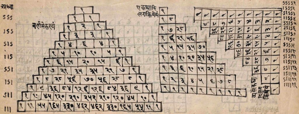
For determining {^n}C_r, Piṅgala describes a practical method named lagakriyā (or galakriyā); the letters la and ga being the first letters of laghu and guru respectively. His description is too terse. Commentators like Halāyudha (c. 950 CE) have explained his method as a pyramidal arrangement of the numerical values of {^n}C_r called Meru-prastāra. It is essentially the same as the famous “Pascal’s triangle” described in Europe in the seventeenth century by P.Herigone (1634 CE) and B.Pascal (1654 CE). The diagram below illustrates this.
Even before Halāyudha, Virahāṅka (c. 600 CE) has described a Meru-prastāra which is almost the same as in Halāyudha. Still earlier, Varāhamihira (c. 550 CE) had described an interesting variant which we describe at the end of this subsection.
Piṅgala’s sūtra 8.34 is usually interpreted as his lagakriyā method; however Jayant Shah argues [19] that the lagakriyā is actually implied in some other sūtra of Piṅgala’s Chandaḥ-sūtra in its Yajur recension (8.23b).
The Indian lagakriyā pyramid (equivalently, Pascal’s triangle) is described in the following diagram. Each row contains all the {^n}C_r‘s for a fixed n, arranged in increasing order of r. 1 is at the vertex of the triangle, the next row has two entries (both 1) corresponding to {^1}C_0 and {^1}C_1, the subsequent row has three entries {^2}C_0=1, {^2}C_1=2, {^2}C_2=1, and so on. The entries in each row are written quickly in terms of the entries of the preceding row, using ^{n+1}C_0 = \; ^{n+1}C_{n+1}= 1 and the recurrence relation ^{n+1}C_r = \; ^{n}C_{r-1} +\; ^{n}C_r.
For instance, the row with entries {^4}C_r is obtained as {^4}C_0=1, {^4}C_1=1+3 (={^3}C_0 +\; ^{3}C_1)=4, {^4}C_2=3+3 (={^3}C_1 +\; ^{3}C_2)=6, etc.
| 1 | |||||||||||||||||||||||||||||||
| 1 | 1 | ||||||||||||||||||||||||||||||
| 1 | 2 | 1 | |||||||||||||||||||||||||||||
| 1 | 3 | 3 | 1 | ||||||||||||||||||||||||||||
| 1 | 4 | 6 | 4 | 1 | |||||||||||||||||||||||||||
| 1 | 5 | 10 | 10 | 5 | 1 | ||||||||||||||||||||||||||
| 1 | 6 | 15 | 20 | 15 | 6 | 1 | |||||||||||||||||||||||||
| 1 | 7 | 21 | 35 | 35 | 21 | 7 | 1 | ||||||||||||||||||||||||
| \!\!\!\!\!\!\vdots |
Meru-prastāra or Pascal’s Triangle for {}^{n}C_r
Meru refers to a “mountain”; thus Meru-prastāra is a diagram which resembles a well-spread-out mountain with a peak, a fitting description of the arrangement.
The crucial principle at the heart of Piṅgala’s Meru-prastāra or Pascal’s triangle is again an algebraic formula: the recurrence relation ^{n+1}C_r = \; ^{n}C_{r-1} +\; ^{n}C_{r}.
We mention an interesting variation of Piṅgala’s Meru-prastāra which occurs in Chapter 77 of Bṛhatsaṁhitā by Varāhamihira (c. 550 CE). The chapter discusses Gandhayukti (perfumery). Verse 20 of this chapter mentions that 1820 combinations can be formed by choosing 4 perfumes from 16 basic perfumes (^{16}C_4=1820). Verse 22 indicates the method for constructing a table which would give the number of such combinations.
We illustrate Varāhamihira’s table. In each column the entries are filled from below to top. The first column lists the ^{n}C_1=n, the natural numbers, from n=1 to n=16. The next column lists the ^{n+1}C_2 (= the sum of natural numbers from 1 to n) from n=1 to n=15. They are filled up successively by diagonal addition using ^{n+1}C_2=\; ^{n}C_2+^{n}C_1, for instance, 3=1+2, 6=3+3, 10=6+4, 15=10+5 etc. The third column lists the ^{n+2}C_3 from n=1 to n=14 using ^{n+1}C_3=\; ^{n}C_3+^{n}C_2, for instance, 4=1+3, 10=4+6, 20=10+10,\ 35=20+15 etc. Similarly the fourth column lists the ^{n+3}C_4 from n=1 to n=13: 5=1+4, 15=5+10, 35=15+20, 70=35+35 and so on, till finally we have the required ^{16}C_4=\; ^{15}C_4+ {}^{15}C_3=1365+455=1820.
| 16 | |||
| 15 | 120 | ||
| 14 | 105 | 560 | |
| 13 | 91 | 455 | 1820 |
| 12 | 78 | 364 | 1365 |
| 11 | 66 | 286 | 1001 |
| 10 | 55 | 220 | 715 |
| 9 | 45 | 165 | 495 |
| 8 | 36 | 120 | 330 |
| 7 | 28 | 84 | 210 |
| 6 | 21 | 56 | 126 |
| 5 | 15 | 35 | 70 |
| 4 | 10 | 20 | 35 |
| 3 | 6 | 10 | 15 |
| 2 | 3 | 4 | 5 |
| 1 | 1 | 1 | 1 |
Varāhamihira’s table for Gandhayukti
One can see that Varāhamihira’s table is simply a suitably rotated version of the Meru-prastāra or Pascal’s Triangle displayed earlier after ignoring the 1’s at the beginning of each row of the latter. To see this, consider the line formed by the second entry in each row of the Meru-prastāra, i.e., all the ^{n}C_1’s from n=1 onwards. The entries are 1,2,3,4,5,6,7,…. Rotate it to make it a vertical column with 1 at the base. Then one gets the first column of Varāhamihira’s table. Likewise, consider the next parallel line in the Meru-prastāra formed by the third entries i.e., the ^{n}C_2’s from n=2 onwards, i.e., 1,3,6,10,15,21,…. Rotating it suitably gives the second column of Varāhamihira’s table.
While Varāhamihira’s table is filled up using the recurrence relation ^{n+1}C_r = \; ^{n}C_{r-1} +\; ^{n}C_{r}, it can be seen that such an arrangement involves the realisation of the algebraic principle
^nC_r=\; ^{n-1}C_{r-1} + ^{n-2}C_{r-1} + \cdots + ^{r-1}C_{r-1}.
Note that the standard textbook formula ^{n}C_r = \frac{n(n-1)(n-2)\cdots (n-r+1)}{1\cdot 2\cdot 3 \cdots r} involves several multiplications and divisions; whereas the algorithms of Piṅgala and Varāhamihira for computing ^{n}C_r, based on ingenious use of algebraic recurrence relations, involve only addition and are thus much simpler for practical computations.
Impact of Piṅgala: Virahāṅka–Fibonacci numbers
The mathematical ideas in Piṅgala’s Chandaḥ-sūtra had a profound impact on the development of numerous combinatorial algorithms and results by post-Vedic Indian mathematicians. It is a vast topic. We briefly mention one combinatorial problem, which arose from the study of metres, and which led to Virahāṅka’s work on what are usually referred to as “Fibonacci numbers”. In his talk on 25.2.2022 mentioned earlier, Manjul Bhargava mentioned the Virahāṅka–Fibonacci sequence as the eighth among the ten fundamental Indian contributions to mathematics that everyone should know.
We first define the “mātrā” of a metre. Assign to each laghu syllable the “mātrā” value 1 and to each guru syllable the “mātrā” value 2. The mātrā of any metrical form is defined to be the sum of the mātrā values of each syllable in the metre.
The mātrā-vṛtta is the analysis (classification etc) of metrical patterns by their mātrā. The topic is briefly touched upon by Piṅgala in Chapter 4 of his treatise and then in Nātyaśāstra of Bharata (c. 200 BCE); it is discussed more elaborately by Virahāṅka in his Prākṛta text Vṛtta-jāti-samuccaya (c. 600 CE) and subsequent prosodists.
A natural question taken up in Indian prosody from at least the time of Virahāṅka is:
Problem. Find the total number of metrical forms V_n with a given mātrā value n.
Clearly V_1=1 and V_2=2. Virahāṅka observes that V_n satisfies the recurrence relation
V_n=V_{n-1}+V_{n-2}. To see this, consider the last syllable c. There are two mutually exclusive possibilities:
- c is laghu, i.e., it has mātrā value is 1. In this case, the sum of the mātrā values of the preceding syllables is n-1. This can happen in V_{n-1} ways.
- c is guru, i.e., it has mātrā value 2. In this case, the sum of the mātrā values of the preceding syllables is n-2. This can happen in V_{n-2} ways.
Hence: V_n = V_{n-1}+V_{n-2}. Natural and beautiful!
Using V_1=1 and V_2=2, the recurrence generates the values for V_n successively:
| n | 1 | 2 | 3 | 4 | 5 | 6 | 7 | 8 | 9 | 10 |
| V_n | 1 | 2 | 3 | 5 | 8 | 13 | 21 | 34 | 55 | 89 |
Virahāṅka sequence V_n
The Piṅgala-inspired Virahāṅka numbers V_n are now known as “Fibonacci numbers” after Leonardo Pisano (c. 1200 CE), nicknamed Fibonacci (meaning, son of Bonacci).
There are other combinatorial problems on mātrā-vṛtta, analogous to Piṅgala’s prastāra, naṣṭa, uddiṣṭa and lagakriyā, discussed by Virahāṅka and subsequent authors.
An anecdote on Piṅgala
Piṅgala is highly venerated in ancient traditions and referred to as a Muni, an Ācārya and a Nāga. Recall that Nāga means serpent as also the best or excellent of any kind. Serpent sometimes symbolizes wisdom, and hence a person endowed with great wisdom could be reverentially mentioned as a Nāga. Legends surrounding Piṅgala appear to indulge in a double entendre involving the word Nāga.
Piṅgala attained legendary fame for his scholarship and brilliance. There is a proverbial simile: “as shrewd as Piṅgala”. It is said of a person who tactfully accomplishes his mission: “He has studied Piṅgala”. There is an interesting story on Piṅgala’s presence of mind which enables him to escape death ([6], p. 75).
After a long journey across mountains and forests, a serene Piṅgala, while on his return journey, was suddenly confronted with Garuḍa, who had enmity with Piṅgala’s family. When the hungry Garuḍa was about to devour him, Piṅgala humbly pleaded with Garuḍa,
Garuḍa got curious and agreed to listen. As Piṅgala began his narration, Garuḍa got fascinated by the Chandaḥśāstra and its mathematical presentations, and listened eagerly.
While explaining the science, Piṅgala kept on drawing long prastāra diagrams directed towards the seashore and in the process steadily moved towards the sea. Through mathematical lines comprising symbols, Piṅgala described the four “yakāra” that are involved in the metre named bhujaṅgaprayāta. This metre, mentioned in Chapter VI Sūtra 43 of Piṅgala’s Chandaḥ-sūtra, too originated in the Ṛgveda. (For instance, the phrase in Ṛgveda X.167.1 : “sahasraṃ ta indrotayo naḥ sahasram”.) Note that bhujaṅga means serpent and prayāta means vanished, departed, gone, etc.,
On reaching the sea, Piṅgala utters “bhujaṅgaprayāta” and escapes into the pātāla (nether world) through the sea route. Even at a critical moment in the face of death, the witty Piṅgala indulges in a pun: mentioning bhujaṅgaprayāta both as the term for a specific metre as well as a statement that the Nāga vanishes.
The above tale not only shows that Piṅgala’s work was held in high esteem, it also shows that mathematics was considered important, charming and interesting. A folklore could be created from a perception that the mathematical aspects of Piṅgala’s treatises were so captivating and absorbing, that they could even be used to distract a sworn enemy from a vengeful act. The story brings out the zest for all-round learning. Garuḍa had lust for food, and lust for revenge; but much more compelling was his lust for knowledge, and that too knowledge of a mathematical flavour!
References
We are not sure whether it will be possible to discuss the rich combinatorial mathematics that developed in post-Vedic India in the present series. We, therefore, give below only a few references.
A concise account of combinatorial algorithms arising in India out of prosody, music and other themes, can be obtained from the following lectures by M.D.Srinivas in the NPTEL course on “Mathematics in India from Vedic Period to Modern Times”: Lecture 5 (Piṅgala’s Chandaḥ-śāstra); Lectures 18 and 19 (Development of Combinatorics in India 1 and 2).
The papers [25] and [19] discuss Piṅgala’s combinatorial work and the paper [26] discusses the Virahāṅka-Fibonacci numbers.
Apart from Indian prosody, the theory of Indian music involves sophisticated combinatorial procedures. The paper [20] discusses combinatorial questions and methods in Indian musicology studied in Saṅgītaratnākara of Sārṅgadeva (c. 1225 CE), a celebrated treatise on music.
Numerous combinatorial results occur in the treatises of post-Vedic Indian mathematicians like Brahmagupta (628 CE), Śrīdharācārya (750 CE), Mahāvīra (850 CE), Bhāskarācārya (1150 CE) and Nārāyaṇa Paṇḍita (c. 1350 CE). The paper [23] illustrates some astonishingly modern approaches in the combinatorial work of Nārāyaṇa Paṇḍita.
Sophisticated algorithms of combinatorial flavour also occur in Indian works on magic squares. It is again a vast topic. Some examples can be seen in [21] and [22].
References
- [1] Sri Aurobindo, The Secret of the Veda, Sri Aurobindo Birth Centenary Library (SABCL) Vol. 10, Sri Aurobindo Ashram, Pondicherry (1972). Originally appeared in the Arya in 24 instalments from August 1914 to July 1916.
- [2] A.L. Basham, The Wonder that was India, Sidgwick and Jackson, London (1954).
- [3] B. Bavare and P.P. Divakaran, Genesis and Early Evolution of Decimal Enumeration: Evidence from Number Names in Ṛgveda, Indian Journal of History of Science 48(4), 535–581 (2013).
- [4] N.L. Biggs, The Roots of Combinatorics, Historia Mathematica 6, 109–136 (1979).
- [5] N.L. Biggs, E.K. Lloyd and R.J. Wilson, The History of Combinatorics, Handbook of Combinatorics Vol. 2 (eds. R. Graham, M. Grötschel and L. Lovász), Elsevier (1995).
- [6] Asoke Chatterjee Sastri, Piṅgalacchandaḥsūtra–A Study, University of Calcutta (1987).
- [7] B. Datta, The Science of the Śulba, University of Calcutta (1932); Cosmo Pub. (1993).
- [8] B. Datta and A.N. Singh, History of Hindu Mathematics Part I, Motilal Banarsidass (1935); reprinted by Asia Publishing House (1962) and Bharatiya Kala Prakashan (2004).
- [9] P.P. Divakaran, Notes on Yuktibhāṣā: Recursive Methods in Indian Mathematics, Studies in the History of Indian Mathematics (ed. C.S. Seshadri), Hindustan Book Agency, New Delhi (2010).
- [10] P.P. Divakaran, What is Indian about Indian Mathematics? Indian Journal of History of Science 51(1), 56–82 (2016).
- [11] P.P. Divakaran, The Mathematics of India: Concepts, Methods, Connections, Hindustan Book Agency, New Delhi (2017).
- [12] A.K. Dutta, Powers of Ten: Genesis and Mystic Significance. Srinvantu 58(2), 44–52 (2008). Reprinted in Mother India LXII(11), 957–967 (2009) \& Vedic Venues 2, 43–56 (2013).
- [13] A.K. Dutta, Kuṭṭaka, bhāvanā and Cakravāla, Studies in the History of Indian Mathematics (ed. C.S. Seshadri), Hindustan Book Agency, New Delhi, 145–199 (2010).
- [14] A.K. Dutta, Decimal System in India, Encyclopaedia of the History of Science, Technology, and Medicine in Non-Western Cultures (ed. H. Selin), Springer (2015).
- [15] A.K. Dutta, Was there sophisticated mathematics during Vedic Age? Platinum Jubilee Memorial Volume, Ramakrishna Mission Vidyamandira, Belur Math, 361–385 (2016).
- [16] A.K. Dutta, The bhāvanā in Mathematics, Bhāvanā 1(1), 13–19 (2017).
- [17] A.K. Dutta, Weighted Arithmetic Mean in Ancient India, Bhāvanā 1(4), 24–36 (2017).
- [18] G. Ifrah, The Universal History of Numbers, John Wiley and Sons (2000).
- [19] J. Shah, A History of Piṅgala’s Combinatorics, Gaṇita Bhāratī 35, 1–54 (2013).
- [20] Raja Sridharan, R.Sridharan and M.D.Srinivas, Combinatorial Methods in Indian Music: Pratyayas in Saṅgītaratnākara of Sārṅgadeva, Studies in the History of Indian Mathematics (ed. C.S. Seshadri), Hindustan Book Agency, New Delhi, 55–112 (2010).
- [21] Raja Sridharan and M.D.Srinivas, Study of Magic Squares in India, Math Unlimited: Essays in Mathematics (eds. R.Sujatha, H.N.Ramaswamy, C. S.Yogananda), Taylor \& Francis, London, 383–391 (2011).
- [22] Raja Sridharan and M.D.Srinivas, Folding Method of Nārāyaṇa Paṇḍita for the Construction of Samagarbha and Viṣama Magic Squares, Indian Journal of History of Science 47, 589–605 (2012).
- [23] Raja Sridharan, R.Sridharan and M.D.Srinivas, Nārāyaṇa Paṇḍita’s enumeration of combinations and associated representations of numbers as sums of binomial coefficients, Indian Journal of History of Science 47, 607–631 (2012).
- [24] Raja Sridharan, R.Sridharan and M.D.Srinivas, Nārāyaṇa’s Generalisation of Mātrā-vṛtta-prastāra and the Generalised Virahāṅka-Fibonacci Representation of Numbers, Indian Journal of History of Science 50(2), 227–244 (2015).
- [25] R.Sridharan, Sanskrit Prosody, Piṅgala Sūtras and Binary Arithmetic, Contributions to the History of Indian Mathematics (ed. G.G. Emch, R. Sridharan, M.D. Srinivas), Hindustan Book Agency, New Delhi (2005).
- [26] R.Sridharan, Pratyayas for Mātrāvṛttas and Fibonacci Numbers, Mathematics Teacher 42, 120–137 (2006).
- [27] Swami Vivekananda, Complete Works, Advaita Ashram, Kolkata (10th ed. 2012).
Footnotes
- The entire poem is reproduced at the end of this article. ↩
- Here and in a few other instances in this text, two sets of page numbers are cited when the translation and interpretation occur in different pages of the reference. ↩
- In Vedic hymns, the Cow is the symbol of consciousness in the form of knowledge and the wealth of cows symbolic of the richness of mental illumination (cf. [1], pp. 114; 42). The sanctified Bricks (iṣṭakā, i.e., that which helps attain the iṣṭa) are charged with, and represent, the mantras (cf. [12]). ↩
- Billion means 10^{12} (million million) in England and Germany but 10^9 (thousand million) in USA and France. Here we use it for 10^{12}. ↩
- On the semigroup of a meromorphic curve I, Proceedings of the International Symposium on Algebraic Geometry, Kyoto 1977 (ed. M. Nagata), Kinokuniya, Tokyo, 249–414 (1978). ↩
- https://www.youtube.com/watch?v=T0gCkyKVQUg. ↩