Introduction
Mathematics in India has a rich and hallowed history. Ancient Indian mathematicians strived to be concise yet clear, cryptic yet compelling in their style and substance. The Śulbasūtras, the oldest extant texts (prior to 800 BCE) explicitly state and make use of the so-called Pythagorean theorem apart from giving various interesting approximations to surds, in connection with the construction of altars and fire-places of different sizes and shapes.
By the time of Āryabhaṭa (c. 499 CE), Indian mathematicians were fully conversant with most of the mathematics that we currently teach at the elementary level in our schools, such as the methods for extracting square root and cube root. Among other things, Āryabhaṭa also presented the differential equation of the sine function in its finite-difference form and a method for solving linear indeterminate equations. The bhāvanā law of Brahmagupta (c. 628 CE) and the cakravāla algorithm described by Jayadeva and Bhāskarācārya (12th century CE) for solving the quadratic indeterminate equation are some of the important landmarks in the evolution of mathematics in India.
Following the era of Āryabhaṭa and Brahmagupta, Indian mathematicians set out to explore the principles, rules and examples under the class of texts in pāṭīgaṇita1 that dealt with select topics in mathematics, mainly comprising of arithmetic, planar geometry and mensuration. There are also topics pertaining to algebra present in this class of texts, where intelligent assumptions and substitutions help arrive at the answers quickly. Śrīdharācārya (c. 750 CE), Mahāvīra (c. 850 CE), Śrīpati (1039 CE), Bhāskarācārya II (c. 1150 CE), and others authored acclaimed texts in pāṭīgaṇita.
The advent of Mādhava (c. 1350 CE) in the Kerala school of astronomy and mathematics ushered in a great impetus in the evolution of mathematical ideas, by enunciating the infinite series for \pi (the so-called Gregory-Leibniz series) and other trigonometric functions. Around the very same time, elsewhere in India, emerged one of the most comprehensive works in pāṭīgaṇita authored by Nārāyaṇa Paṇḍita.
Nārāyaṇa Paṇḍita is a fourteenth century Indian mathematician, whose elaborate and comprehensive pāṭīgaṇita text is titled Gaṇitakaumudī. The number of verses in this text is close to 930, which is almost three times the famous work Līlāvatī of Bhāskarācārya. The content and the range of topics covered are also richer than in Līlāvatī. Through these works, Indian mathematicians not only made breakthroughs in mathematics but also displayed creative prowess in presenting their ideas through fascinating poetry. Thus what we find in these works is a beautiful blend of mathematics, poetry as well as useful pedagogical techniques. Nārāyaṇa Paṇḍita too showed remarkable ingenuity in his clear enunciation of rules, fascinating propositions, captivating puzzles, and nuanced formulations.
However, the number of available manuscripts of his work is very small and the entire text came to light only in recent times. Therefore the present text provides an excellent opportunity to study the work carefully, and reflect on the salient mathematical developments of the time. The authors of this article are currently engaged in bringing out a revised edition, with translation, and a detailed mathematical exposition of the contents of Gaṇitakaumudī.
Here, we present key details about the text, its contents and the author, and also highlight certain unique contributions contained in it. While the article showcases only a handful of interesting verses from Gaṇitakaumudī, Nārāyaṇa Paṇḍita’s adeptness makes a compelling case for this text to be considered as an important work.
About the Gaṇitakaumudī and its author
The content of this text in its entirety came to light only in the early twentieth century, thanks to the efforts of Pandit Padmakara Dvivedi, the son of the famous scholar Pandit Sudhakara Dvivedi whose contribution to the field of astronomy and mathematics is phenomenal.
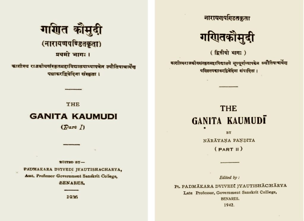
In his preface to an edition brought out in two parts, Padmakara Dvivedi mentions [9], [p. i] that he accidentally discovered a complete manuscript of Gaṇitakaumudī in his father’s collection and, by looking into its contents, he decided to bring out an edited version of the work. The two volumes, [8] and [9], were brought out in the years 1936 and 1942. Dvivedi conjectures that this work must have intended to be an alternative to the widely known Līlāvatī of Bhāskarācārya from the twelfth century CE. Apart from Gaṇitakaumudī, Bījagaṇitāvataṃśa is the only other work known to be authored by Nārāyaṇa Paṇḍita, with just one incomplete manuscript available in Benares (see [5], [p. 388] and [17], [p. i]).
Paramanand Singh brought out translations of certain chapters of the Gaṇitakaumudī as a series of publications [11] [12] [13] from 1998 to 2002 (see also [10]). However, an in-depth study and a more detailed mathematical account need to be undertaken to showcase the mathematical ingenuity in this work of Nārāyaṇa Paṇḍita. The present paper intends to provide a glimpse of the foundational topics in mathematics treated in Gaṇitakaumudī, or `the moonlight of mathematics’.
Reference to Nārāyaṇa Paṇḍita in other works
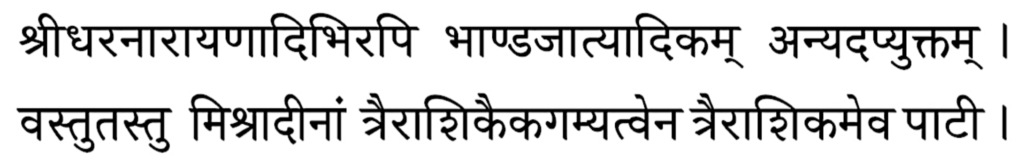
The earliest known allusion to Nārāyaṇa Paṇḍita is in Buddhivilāsinī, a well-known commentary to the famous text Līlāvatī of Bhāskaracārya. Buddhivilāsinī was authored by Gaṇeśa Daivajña in 1546 CE. In this work, Gaṇeśa Daivajña, while referring to the contributions of different authors to certain topics in mathematics, cites Śrīdhara and Nārāyaṇa as propounders of mathematical aspects that deal with barter, trade and mixed proportions, which primarily involve the application of Trairāśika, or the `rule of three’. The following (see [1], [p. 6.]) is the aforementioned quote from Buddhivilāsinī.
|
śrīdhara-nārāyaṇādibhirapi bhāṇḍajātyādikam anyat apyuktam\vert vastutastu miśrādīnāṃ trairāśikaika-gamyatvena trairāśikam eva pāṭī\vert |
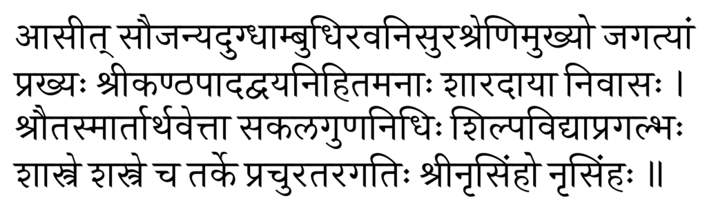
Unfortunately, not much is known about Nārāyaṇa Paṇḍita’s date of birth, whereabouts and other biographical details. Only very little information is provided by him in his verses towards the end of the text. One verse, in the Sragdharā metre, reflecting on the great scholarship of his father, is as follows:
|
āsīt saujanya-dugdhāmbudhiravanisura-śreṇimukhyo jagatyāṃ prakhyaḥ śrīkaṇṭhapādadvaya-nihitamanāḥ śāradāyā nivāsaḥ\vert śrauta-smārtārthavettā sakalaguṇa-nidhiḥ śilpavidyā-pragalbhaḥ śāstre śastre ca tarke pracuratara-gatiḥ śrīnṛsiṃho nṛsiṃhaḥ\Vert |
From the above verse, we understand that Nārāyaṇa Paṇḍita’s father was Nṛsiṃha and that he was an outstanding scholar in several branches of knowledge. Besides this, no other biographical details of Nārāyaṇa Paṇḍita are known. Apart from Gaṇitakaumudī, Bījagaṇitāvataṃśa is the only other work known to be authored by Nārāyaṇa Paṇḍita, with just one incomplete manuscript available in Benares (see [5], [p. 388] and [17], [p. i]).
Date of composition of Gaṇitakaumudī
The date of composition of Gaṇitakaumudī is given by Nārāyaṇa Paṇḍita himself in the following verse that appears in the Āryā metre at the end of the text.
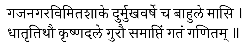
|
gajanagaravi-mitaśāke durmukhavarṣe ca bāhule māsi\vert dhātṛtithau kṛṣṇadale gurau samāptiṃ gataṃ gaṇitam\Vert |
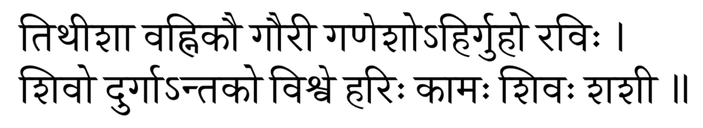
Thus, we unambiguously know that the Gaṇitakaumudī was completed in the year 1356 CE. It is interesting to note that Nārāyaṇa Paṇḍita has specified the tithi count in terms of the devatā of the tithi. Though the texts on mathematical astronomy (siddhānta-granthas) do not present the list of devatās associated with the tithis, the muhūrta texts do so. For instance, in the text Muhūrtacintāmaṇi we have the following verse right at the beginning (v. 3) of the text.
|
tithīśā vahnikau gaurī gaṇeśo\acute{\;}hirguho raviḥ\vert śivo durgā\acute{\;}ntako viśve hariḥ kāmaḥ śivaḥ śaśī\Vert |
Here starting from `vahni‘ up to `śaśī‘ we have 15 names listed. These are the deities (devatās) associated with the 15 tithis commencing from prathamā to pūrṇimā. The devatā for the second tithi (dvitīyā) is mentioned to be `ka‘ here. One the meanings of `ka‘ is Brahmā, which is a synonym of dhātṛ. Thus dhātṛtithi corresponds to dvitīyā.
Contents, structure, and significance of Gaṇitakaumudī
The Gaṇitakaumudī contains fourteen chapters in all. The chapters are called vyavahāras, with about 547 sūtra verses and 385 udāharaṇa verses. While most of the verses composed by Nārāyaṇa are in the Āryā metre, Bhāskara employs a variety of other charming metres for composing verses.
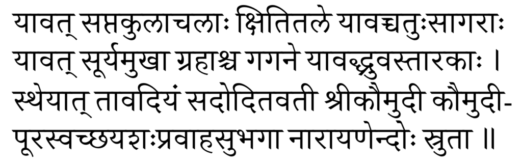
In a verse in the Śārdūlavikrīḍita metre towards the end of his work, Nārāyaṇa Paṇḍita expresses his wish that it shall attain widespread acceptance and popularity.
|
yāvat saptakulācalāḥ kṣititale yāvaccatuḥsāgarāḥ yāvat sūryamukhā grahāśca gagane yāvaddhruvastārakāḥ\vert stheyāt tāvadiyaṃ sadoditavatī śrīkaumudī kaumudī- pūrasvaccha-yaśaḥpravāha-subhagā nārāyaṇendoḥ srutā\Vert |
This verse is a beautiful piece of poetry in itself. It has a lot of poetic flourishes (ala\dot{n}kāras) like rūpaka, vyatireka, about which we do not elaborate as they are beside the scope of this paper.
The nature of the foundational mathematics dealt with in this text, including the special chapter on magic squares, indeed makes it a sought-after repository of Indian mathematical heritage. Nārāyaṇa Paṇḍita has also written his own short commentary, called Vāsanā, which succinctly presents explanation to the sūtras, or rules, and solutions to the examples. Table 1 presents a brief summary of the contents of Gaṇitakaumudī.
| No. | Chapter Title | Mathematical topics covered |
| 1 | Prakīrṇaka-vyavahāraḥ | Logistics, weights and measures |
| 2 | Miśraka-vyavahāraḥ | Partnership, sales, interest, etc. |
| 3 | Śreḍhī-vyavahāraḥ | Sequences and series |
| 4 | Kṣetra-vyavahāraḥ | Geometry of planar figures |
| 5 | Khāta-vyavahāraḥ | Excavations |
| 6 | Citi-vyavahāraḥ | Problems pertaining to stacks |
| 7 | Rāśi-vyavahāraḥ | Mounds of grain |
| 8 | Chāyā-vyavahāraḥ | Shadow problems |
| 9 | Kuṭṭakam | Linear indeterminate equations |
| 10 | Vargaprakṛtiḥ | Quadratic indeterminate equations |
| 11 | Bhāgādānam | Factorisation |
| 12 | Aṃśāvatāraḥ | Partitioning unity into unit-fractions |
| 13 | A\dot{n}kapāśaḥ | Combinatorics |
| 14 | Bhadragaṇitam | Magic squares: Theory & Construction |
Highlights from Gaṇitakaumudī
By virtue of being the largest among the extant pāṭīgaṇita works, Gaṇitakaumudī contains a gamut of wide-ranging topics and unique sections, approaches, and illustrative puzzles. In this section, we highlight a few select topics and verses that may interest general readers, and delight the math-enthusiasts and connoisseurs of the history of mathematics alike. We start with a couple of captivating examples that Nārāyaṇa provides in order to illustrate the application of mathematical rules and principles.
Captivating examples
The Līlāvatī of Bhāskarācārya is generally known for its beautiful examples. In his Gaṇitakaumudī work, Nārāyaṇa demonstrates a similar prowess. While dealing with the elaborate twenty-one varieties of quadratic equations, he presents a variety of fascinating and practical examples, by employing beautiful metres to compose verses. These verses not only exemplify his creative mind, but also his mastery of Sanskrit poetry. Let us present a couple of samples which are in the Śārdūlavikrīḍita metre.
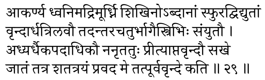
|
ākarṇya dhvanimadrimūrdhni śikhino\acute{\;}bdānāṃ sphuradvidyutāṃ vṛndārdhatrilavau tadantaracaturbhāgaistribhiḥ saṃyutau\vert adhyardhaikapadādhikau nanṛtatuḥ prītyāptavṛndau sakhe jātaṃ tatra śatatrayaṃ pravada me tatpūrvavṛnde kati\Vert 29 \Vert |
This is an example of viśleṣamūlajāti, which is a technical term referring to one of the varieties of quadratic equations given in the text. We do not venture to explain the term here (or in the next example), as it is not quite germane to the paper.
Let x be the number of peacocks in the `earlier’ group at the top of the hill. Now, the problem states that another group joined this group on hearing the sound made by the clouds. The description given in the verse amounts to solving the following equation for x.
\[\begin{align*}
x + \frac{1}{2} x + \frac{1}{3} x + \frac{3}{4} \left(\frac{1}{2} – \frac{1}{3}\right) x + \frac{3}{2} \sqrt{x} &= 300\\
\frac{47}{24} x + \frac{3}{2} \sqrt{x} &= 300\end{align*}\]This equation is similar to the equation ax \pm b\sqrt{x} = c with a = \frac{47}{24}, b = \frac{3}{2}, and c = 300. We use the formula stated by Nārāyaṇa to find the value of x.
\[\begin{align*}
x &= \left(\frac{\sqrt{b^2 + 4ac} – b}{2a}\right)^2\\
& = \left(\frac{\sqrt{\left(\frac{3}{2}\right)^2 + 4 \times \frac{47}{24} \times 300} – \frac{3}{2}}{2 \times \frac{47}{24}}\right)^2= 144\end{align*}\]Thus we find that the number of peacocks that were present in the previous group is 144.
To illustrate the principle of śeṣamūlajāti, Nārāyaṇa brings forth yet another beautiful example.
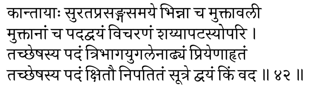
|
kāntāyāḥ surataprasa\dot{n}gasamaye bhinnā ca muktāvalī muktānāṃ ca padadvayaṃ vicaraṇaṃ śayyāpaṭasyopari\vert taccheṣasya padaṃ tribhāgayugalenāḍhyaṃ priyeṇāhṛtaṃ taccheṣasya padaṃ kṣitau nipatitaṃ sūtre dvayaṃ kiṃ vada\Vert 42 \Vert |
The problem posed here when expressed in algebraic notation amounts to:
\[\begin{align}
\label{eq:e1}
x – b_1 \sqrt{x} – b_2 \sqrt{(x – b_1 \sqrt{x})}
– b_3 \sqrt{x – b_1 \sqrt{x} – b_2 \sqrt{(x – b_1 \sqrt{x})}} … = c
\end{align}\]where, b_1, b_2, b_3 are parameters whose values are provided in the problem statement and x is the unknown whose value is to be determined. Further, on making the substitutions x - b_1 \sqrt{x} = y; y - b_2 \sqrt{y} = z, the equation above reduces to:
\[\begin{equation}
\label{eq:e2}
z – b_3 \sqrt{z} = c
\end{equation}\]Applying the formula given by Nārāyaṇa, we first get the value of z, then the value of y, and then of x, which is the desired result.
Substituting the parametric values as per the description given in the verse for 1, we get
\[\begin{equation}
\label{eq:e3}
x – \left(2 \sqrt{x} – \frac{1}{4} \sqrt{x}\right) – \left(\sqrt{y} + \frac{2}{3} \sqrt{y}\right) – \sqrt{z} = 2
\end{equation}\]where,
\[\begin{equation}
\label{eq:q1}
y = x – \left(2 \sqrt{x} – \frac{1}{4} \sqrt{x}\right) = x – \frac{7}{4} \sqrt{x}
\end{equation}\]and
\[\begin{equation}
\label{eq:q2}
z = y – \left(\sqrt{y} + \frac{2}{3} \sqrt{y}\right) = y – \frac{5}{3} \sqrt{y}.
\end{equation}\]Thus, equation \eqref{eq:e2} becomes
\[\begin{equation}
\label{eq:q3}
z – \sqrt{z} = 2.
\end{equation}\]Solving \eqref{eq:q3}, we first obtain the value of z to be 4. Now, plugging this value in \eqref{eq:q2}, we find that y = 9. Using this value of y in \eqref{eq:q1}, we get x = 16.
Thus we find that there were 16 pearls present in the necklace before it broke.
What we found above is an example where we had to solve nested quadratic equations. As mentioned before, this section dealing with twenty-one varieties of quadratic equations presents very beautiful examples, sometimes multiple, for each variety. Many of these varieties are not found in Līlāvatī and other earlier works. Thus, by bringing forth subtler varieties of quadratic equations with such captivating examples, Nārāyaṇa demonstrates his excellent creativity.
A mathematical riddle
One of the purposes of doing mathematics is to find solutions to a variety of problems encountered on a day-to-day basis. That it can be pursued purely for intellectual fun has also been demonstrated by Nārāyaṇa in a few sections in his Gaṇitakaumudī. From one such section named ghātasamāsādi-sāmyam, we present a verse containing sixfold riddles.
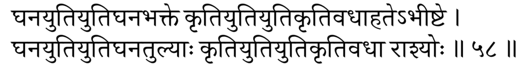
ghanayutiyutighanatulyāḥ kṛtiyutiyutikṛtivadhā rāśyoḥ\Vert 58 \Vert
It may be noted that in the verse above, a single syllable `ti‘ appears 12 times. Combined with another syllable in the form of `yuti,’ it appears 8 times. Similarly, we find the words `kṛti‘ and `ghana‘ appearing 4 times each with a certain symmetry. It is certainly not an easy task to come up with such compositions which carry a lot of literary charm.
That said, the riddle posed by Nārāyaṇa is to find numbers x and y so that the following six equations are satisfied independently.
\[\begin{array}{llll}
1. & x^3 + y^3 & = & x^2 + y^2 \\
2. & x^3 + y^3 & = & (x + y)^2 \\
3. & x^3 + y^3 & = & x\cdot y \\
4. & (x + y)^3 & = & x^2 + y^2 \\
5. & (x + y)^3 & = & (x + y)^2 \\
6. & (x + y)^3 & = & x\cdot y \\
\end{array}\]Considering two numbers a and b, it can be easily verified that the following solutions satisfy the above equations.
\[\begin{array}{llllllll}
1. & x & = & \frac{a\, (a^2 + b^2)}{a^3 + b^3}; & & y & = & \frac{b\, (a^2 + b^2)}{a^3 + b^3} \\
2. & x & = & \frac{a\, (a + b)^2}{a^3 + b^3}; & & y & = & \frac{b\, (a + b)^2}{a^3 + b^3} \\
3. & x & = & \frac{a\cdot ab}{a^3 + b^3}; & & y & = & \frac{b\cdot ab}{a^3 + b^3} \\
4. & x & = & \frac{a\, (a^2 + b^2)}{(a + b)^3}; & & y & = & \frac{b\, (a^2 + b^2)}{(a + b)^3} \\
5. & x & = & \frac{a\, (a + b)^2}{(a + b)^3}; & & y & = & \frac{b\, (a + b)^2}{(a + b)^3} \\
6. & x & = & \frac{a\cdot ab}{(a + b)^3}; & & y & = & \frac{b\cdot ab}{(a + b)^3} \end{array}\]
Meeting of messengers
That the speed of an object is essentially the distance travelled divided by the time taken is a well-known fact from ancient times, and problems of this kind can be seen even in the Āryabhaṭīya (c. 499 CE). Towards the end of the Gaṇitapāda (v. 31), Āryabhaṭa gives two formulae that give the time that is yet to elapse or that has elapsed since the meeting of two messengers moving with two different speeds. Here, the two cases correspond to the messengers (or in general any two objects) moving in opposite directions or the same direction. The importance of such problems cannot be overstated considering the fact that walking (pādayātrā) was about the only mode of travelling possible to a common man in those days.
What is special about Nārāyaṇa Paṇḍita in dealing with this class of problems is the segregation that he brings in. He divides this section into two parts; one considering the path to be linear and the other considering it to be circular. He then gives two different formulae. The following verse presents the formula for the linear case.
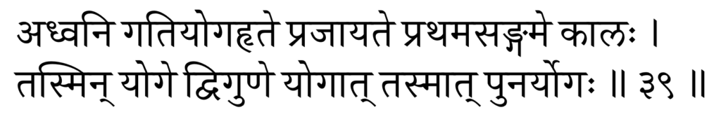
|
adhvani gatiyogahṛte prajāyate prathamasa\dot{n}game kālaḥ\vert tasmin yoge dviguṇe yogāt tasmāt punaryogaḥ\Vert 39 \Vert |
Let the speeds of the two travellers be v_1 and v_2 respectively, and the initial distance between them be d. Also, let the time required for their first and second meetings be denoted by t_1 and t_2 respectively. Here, the times of their first meeting (on their paths between two places, in opposite directions) and the second (while returning) are given by:
\[\begin{equation}
\label{eq:e4}
t_{1} = \frac{d}{v_{1} + v_{2}} \quad \mbox{and} \quad t_{2} = \frac{2d}{v_{1} + v_{2}}
\end{equation}\]Nārāyaṇa illustrates this case with a practical example.
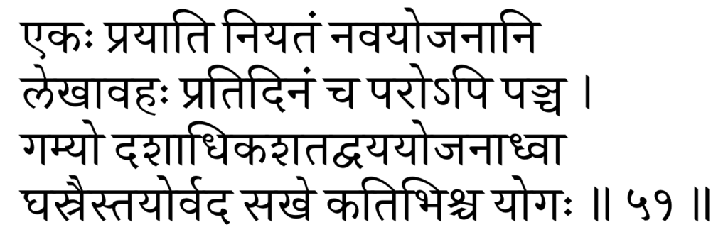
|
ekaḥ prayāti niyataṃ navayojanāni lekhāvahaḥ pratidinaṃ ca paro’pi pañca\vert gamyo daśādhikaśatadvayayojanādhvā ghasraistayorvada sakhe katibhiśca yogaḥ\Vert 51 \Vert |
Time required for their first meeting = \frac{210}{9 + 5} = 15 days.
Time required for their second meeting = 2 \times 15 = 30 days.
Considering the case of a circular path, Nārāyaṇa presents the following rule.

Let the speeds of the two travellers be v_1 and v_2, and c be the circumference of the circular path. Then the time t required for their meeting is given by
\[\begin{equation}
\label{eq:e5}
t = \frac{c}{v_1 ∽ v_2}
\end{equation}\]Here the notation `\backsim‘ denotes the difference between the two speeds.
This equation has an important application in astronomy. As seen from the earth, both the sun and the moon are moving around it. However, the moon moves much faster than the sun and completes its orbit in just 27.33 days, whereas the sun takes about 365.25 days. By using these figures one can calculate their angular speeds and thereby get the duration of what is called the average3 period of a lunar month. This is essentially the average time interval between two successive new moon days (amāvasyas).
Nārāyaṇa illustrates the application of \eqref{eq:e5} with the following example.
|
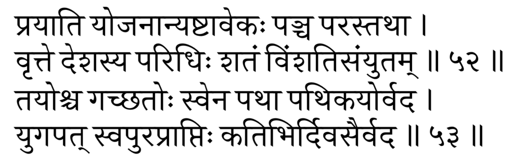
prayāti yojanānyaṣṭāvekaḥ pañca parastathā\vert vṛtte deśasya paridhiḥ śataṃ viṃśatisaṃyutam\Vert 52 \Vert tayośca gacchatoḥ svena pathā pathikayorvada\vert yugapat svapuraprāptiḥ katibhirdivasairvada\Vert 53 \Vert |
By plugging in the values given in the verse in \eqref{eq:e5}, we find that the time required for their meeting = \frac{120}{8-5} = 40 days.
Gosa\dot{n}khyā – Population of cows
The third chapter of Gaṇitakaumudī, namely Śreḍhı̄-vyavahāraḥ is devoted to progressions. Here, Nārāyaṇa introduces a novel section on the estimation of the population of cows. This serves as a classic example for the application of a mathematical principle (finding the sum of sums) in the context of understanding how the cow-population can in principle grow. Nārāyaṇa Paṇḍita’s creative prowess is in full display while presenting this interesting case that is drawn from the experiences of daily life.
In a hypothetical case where a cow begets a female calf every year, and so too her female calf after a few years of its age, Nārāyaṇa directs us to handle this mathematical problem effectively by employing the principle of the sum of sums. The rule for finding the sum of sums to various orders is presented in the following verse:
|
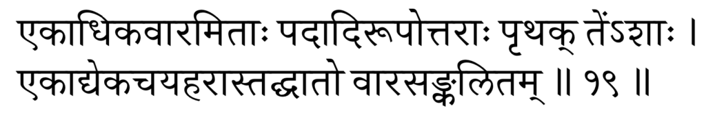
ekādhikavāramitāḥ padādirūpottarāḥ pṛthak te’ṃśāḥ\vert ekādyekacayaharāstadghāto vārasa\dot{n}kalitam\Vert 19 \Vert |
Here the term `pada‘ refers to the number of terms (n) in the arithmetic progression. The term `vāra‘ is used here for the number of times the same mathematical operation (i.e., finding sums) is being repeated. For convenience, we use the word `order’ to refer to this `vāra.’ In the zeroth order, we take every element of the progression to be 1, and denote the sum as v_n^{(0)}. This is given by,
\[\begin{equation}
\label{eq:e6}
v_n^{(0)} = 1 + 1 + 1 + \cdots + 1 = n
\end{equation}\]The first order vārasa\dot{n}kalita denoted by v_n^{(1)} is given by
\[\begin{align}
v_n^{(1)} &= v_1^{(0)} + v_2^{(0)} + v_3^{(0)} + \cdots + v_n^{(0)}\nonumber\\
&= 1 + 2 + 3 + \cdots + n = \frac{n \,(n + 1)}{2} \label{eq:e7}
\end{align}\]The second order vārasa\dot{n}kalita denoted by v_n^{(2)} is given by
\[\begin{align}
v_n^{(2)} &= v_1^{(1)} + v_2^{(1)} + v_3^{(1)} + \cdots + v_n^{(1)}\nonumber\\
&= \frac{1 \,(1 + 1)}{2} + \frac{2 \,(2 + 1)}{2} + \frac{3 \,(3 + 1)}{2}+ \nonumber\\
&\qquad\qquad + \cdots + \frac{n \,(n + 1)}{2}\nonumber\\
&= \frac{n \,(n + 1) \,(n + 2)}{1\cdot 2\cdot 3}\label{eq:e8}
\end{align}\]In general, the kth order vārasa\dot{n}kalita v_n^{(k)} is given by
\[\begin{align}
v_n^{(k)} &= v_1^{(k – 1)} + v_2^{(k – 1)} + v_3^{(k – 1)} + \cdots + v_n^{(k – 1)}\nonumber\\
&= \frac{n \,(n + 1) \,(n + 2) \cdots (n + k)}{1\cdot2\cdot3 \cdots (k + 1)}\label{eq:e9}
\end{align}\]It is essentially this result that Nārāyaṇa has given as vārasa\dot{n}kalita.
\[\begin{equation}
vārasa\dot{n}kalita
= \frac{n}{1}\cdot\frac{n + 1}{2}\cdot\frac{n + 2}{3}\cdot\frac{n + 3}{4} \cdots \frac{n + k}{k + 1}
\end{equation}\]Having presented the above formula, and some more complex ones, Nārāyaṇa provides a brief description of how to tackle a problem pertaining to cow population in the following verses:
|
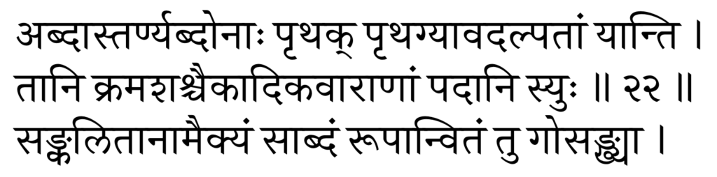
abdāstarṇyabdonāḥ pṛthak pṛthagyāvadalpatāṃ yānti\vert tāni kramaśaścaikādikavārāṇāṃ padāni syuḥ\Vert 22 \Vert sa\dot{n}kalitānām aikyaṃ sābdaṃ rūpānvitaṃ tu gosa\dot{n}khyā\vert |
In this method, the number of years, from which a cow starts begetting a calf, is subtracted from the given number of years. And the same is subtracted from the remainder successively till the remainder becomes smaller than the years that a cow starts reproducing. These remainders are considered as the number of terms. Using the following formula, the first sum of sums is found for the first remainder, the second sum of sums for the second remainder, and so on.
Then Nārāyaṇa poses a puzzle for us to apply and solve the same.
|
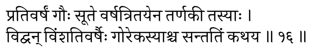
prativarṣaṃ gauḥ sūte varṣatritayena tarṇakī tasyāḥ\vert vidvan viṃśativarṣaiḥ gorekasyāśca santatiṃ kathaya\Vert 16 \Vert |
Given that the number of years is 20, and the number of years required for a cow to beget a calf is 3, we could generate the numbers that are needed to get the sum of sums, as directed by Nārāyaṇa.
\[\begin{align*}
20-3 &= 17 & &\mbox{First sum of sums} && = &&\frac{17}{1} \times \frac{17 + 1}{2} = 153 \\
17-3 &= 14 && \mbox{Second sum of sums} && = &&\frac{14}{1} \times \frac{14 + 1}{2} \times \frac{14 + 2}{3} = 560 \\
14-3 &= 11 && \mbox{Third sum of sums} && = &&\frac{11}{1} \times \frac{11 + 1}{2} \times \frac{11 + 2}{3} \times \frac{11 + 3}{4} = 1001 \\
11-3 &= 8 && \mbox{Fourth sum of sums} && = &&\frac{8}{1} \times \frac{8 + 1}{2} \times \frac{8 + 2}{3} \times \frac{8 + 3}{4} \times \frac{8 + 4}{5} = 792 \\
8-3 &= 5 && \mbox{Fifth sum of sums} && = &&\frac{5}{1} \times \frac{5 + 1}{2} \times \frac{5 + 2}{3} \times \frac{5 + 3}{4} \times \frac{5 + 4}{5} \times \frac{5 + 5}{6} = 210 \\
5-3 &= 2 && \mbox{Sixth sum of sums} && = &&\frac{2}{1} \times \frac{2 + 1}{2} \times \frac{2 + 2}{3} \times \frac{2 + 3}{4} \times \frac{2 + 4}{5} \times \frac{2 + 5}{6} \times \frac{2 + 6}{7} = 8
\end{align*} \]
Progeny of a cow in 20 years = 153 + 560 + 1001 + 792 + 210 + 8 + 20 + 1 = 2745
This is one among the very fascinating puzzles devised by Nārāyaṇa in this text. This class of problems is unique to this text and deserves much attention. It is also highly useful from a pedagogical viewpoint.
Cyclic quadrilaterals and the third diagonal
It is quite interesting to note that nearly one-fourth of the verses in the entire text of Gaṇitakaumudī is present in its fourth chapter Kṣetra-vyavahāra—devoted to geometry—thus making it the biggest of the fourteen chapters. And within the 243 verses of Kṣetra-vyavahāra, Nārāyaṇa Paṇḍita deals with cyclic quadrilaterals, spread over one-third of the chapter.
With 80+ verses, it presents a nuanced and systematic exposition of cyclic quadrilaterals, along with a detailed discussion of its key properties. In his creative mathematical approach, Nārāyaṇa fashions a “third diagonal” by interchanging two sides of a cyclic quadrilateral. Then he provides the precise mathematical expression for getting the magnitude of the third diagonal in terms of its sides. He also provides a precise mathematical relation that enables one to express the area, altitude, and circumradius involving the third diagonal.
Amongst the Indian mathematical texts which have been edited and published so far, nowhere do we find the concept of “third diagonal” enunciated, until the time of Nārāyaṇa Paṇḍita. None of the five important treatises on mathematics authored between Brahmagupta (7th century CE) and Nārāyaṇa (14th century CE)—the pāṭīgaṇita and Triśatikā of Śrīdhara, the Gaṇitasārasa\dot{n}graha of Mahāvīra, the Gaṇitatilaka of Śrīpati and Līlāvatī of Bhāskara II—have the mention of a “third diagonal”, though some of them present certain mathematical results pertaining to cyclic quadrilaterals. We also find Nārāyaṇa Paṇḍita critiquing the formula of circumradius, given by Brahmagupta as not being applicable in general. Thus one can infer that Nārāyaṇa Paṇḍita’s “third diagonal” is novel to the Indian mathematical tradition, and the numerous properties that he presents applying it are nowhere to be found in earlier works.
Taking note of this, Sarasvati Amma in her treatise [15], [p. 96] observes:
The formula involving the “third diagonal” in finding the area of a cyclic quadrilateral as given by Nārāyaṇa Paṇḍita is also found in the later sixteenth century Malayalam text Gaṇitayuktibhāṣā of Jyeṣṭhadeva (see [14], [p. 111]). Nonetheless, Gaṇitakaumudī also employs the notion of the “third diagonal”, to arrive at many more properties of the cyclic quadrilateral. Just like the ingenious mathematician Brahmagupta, Nārāyaṇa Paṇḍita too has impressive results, and his systematic approach to a progressive presentation of mathematical ideas deserves due appreciation.
Nārāyaṇa Paṇdita begins his exposition by first stating the formulae for the diagonals of a cyclic quadrilateral.
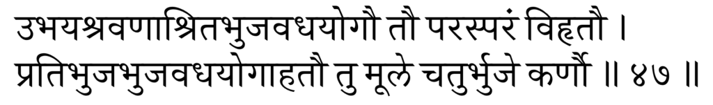
|
ubhayaśravaṇāśritabhujavadhayogau tau parasparaṃ vihṛtau\vert pratibhujabhujavadhayogāhatau tu mūle caturbhuje karṇau\Vert47\Vert |

\[\begin{align}
\label{eq:d1}
d_1 &= \sqrt{\frac{(s_1s_4 + s_2s_3)}{(s_1s_2 + s_3s_4)} \times (s_1s_3 + s_2s_4) }\\
\label{eq:d2}
d_2 &=\, \sqrt{\frac{(s_1s_2 + s_3s_4)}{(s_1s_4 + s_2s_3)} \times (s_1s_3 + s_2s_4) }
\end{align}\]The following verses present the concept of the third diagonal, conditions under which it occurs, its mathematical expression in terms of the sides, and similar considerations.
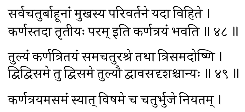
|
sarvacaturbāhūnāṃ mukhasya parivartane yadā vihite\vert karṇastadā tṛtīyaḥ param iti karṇatrayaṃ bhavati\Vert 48 \Vert tulyaṃ karṇatritayaṃ samacaturaśre tathā trisamadoṣṇi\vert dvidvisame tu dvisame tulyau dvāvasadṛśaścānyaḥ\Vert 49 \Vert karṇatrayamasamaṃ syāt viṣame ca caturbhuje niyatam\vert |

with the sides s3 and s4 interchanged, and the third diagonal d3.
In this verse, Nārāyaṇa instructs to swap the face of a cyclic quadrilateral with any of its flank sides. This can also be understood to imply the interchange of the arc lengths corresponding to the chords of the circle which form the sides of the cyclic quadrilateral. The resulting cyclic quadrilateral would have one of the diagonals retained, as a pair of sides is unchanged; and a new diagonal appearing between the interchanged sides as indicated in Figure 2. Based on his previous verse, giving mathematical expressions for the diagonals, the formula for the “third diagonal” can be written as:
\[\begin{equation}
\label{eq:d3}
d_3 \,=\, \sqrt{\frac{(s_1s_2 + s_3s_4)\,(s_1s_4 + s_2s_3)}{(s_1s_3 + s_2s_4)}}
\end{equation}\]It is indeed an illuminating engagement to visualize all the possibilities of the parivartana in cyclic quadrilaterals by fixing the base and mutually interchanging the other three sides. We illustrate six possibilities in Figure 3. When the base itself gets swapped, what it amounts to is the rotation of one of these six possibilities presented in Figure 2.

Following the definition of the third diagonal, Nārāyaṇa presents three propositions on the nature of the third diagonal that has to do with the type of the quadrilateral that the circle circumscribes. These three propositions are listed below:
- The three diagonals are all equal in an equilateral or an equi-trilateral cyclic quadrilateral.
- Two diagonals are equal and the other is unequal in an equi-dichastic or an equi-bilateral cyclic quadrilateral.
- No diagonals are equal in an inequilateral cyclic quadrilateral.
The validity of the first two propositions can be easily verified by making suitable substitutions in \eqref{eq:d3}. The third proposition can be verified by invoking the proof of contradiction assuming that two diagonals are equal. That would enforce two sides to be equal as well. Hence it shows that all three diagonals in an inequilateral cyclic quadrilateral are different (asamaṃ syāt).
As mentioned earlier, Nārāyaṇa utilizes the third diagonal’s relationship to arrive at numerous other results including the area of the cyclic quadrilateral, its circumradius, length of the segments of the diagonals from the point of intersection, altitudes in the cyclic quadrilateral, areas of the component triangles formed by the diagonals within the cyclic quadrilaterals and so on. All along, he presents the rules in a sequence interspersed with the lemmas that would be needed to prove his results. The logical and structural approach to any topic dealt within Gaṇitakaumudī is certainly a hallmark of Nārāyaṇa Paṇḍita!
Turagagati method for generating 4\times4 pandiagonal magic squares
The earliest extant mathematical text in India that presents some detailed treatment on the topic of magic squares is Gaṇitasārakaumudī of the Jaina mathematician Thakkura Pherū (c. 1300 CE). A more detailed mathematical treatment, by way of exclusively devoting a chapter (Chapter 14, consisting of 72 verses), is provided by Nārāyaṇa Paṇḍita in Gaṇitakaumudī.
In this chapter Nārāyaṇa Paṇḍita introduces the principles governing the construction of magic squares, and expounds general methods to construct different forms of magic squares by broadly classifying them into three types. They are:
- Samagarbha (even square of the type 4n \times 4n)
- Viṣamagarbha (even square of the type (4n+2) \times (4n+2))
- Viṣama (odd square of the type (4n \pm 1) \times (4n \pm 1))
where n = 1, 2, 3, ....
Having classified the squares, the first thing Nārāyaṇa does is to point out the connection between magic squares and the arithmetic progression. While doing so, he notes that any sequence in an arithmetic progression can be used to construct magic squares. From the list of contents, as summarized by K.S. Shukla, we come to understand that this chapter includes:
- The method of the Turagagati or horse move for the construction of a 4n \times 4n square.
- The method of superposition for the construction of 4n \times 4n squares.
- The method of equi-spacing for the construction of (4n + 2) \times (4n + 2) squares.
- The method of superposition for odd squares.
- A special method for odd squares.
- The construction of a magic rectangle (vitāna or canopy).
- The construction of magic circles, triangles, hexagons and various other figures, such as the altar, the diamond, etc.
The following verses describe Nārāyaṇa Paṇḍita’s method to construct 4 \times 4 pandiagonal magic squares with an arithmetic progression.
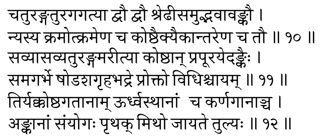
|
catura\dot{n}ga-turagagatyā dvau dvau śreḍhīsamudbhavāva\dot{n}kau\vert nyasya kramotkrameṇa ca koṣṭhaikyaikāntareṇa ca tau\Vert 10 \Vert savyāsavya-tura\dot{n}gamarītyā koṣṭhān prapūrayeda\dot{n}kaiḥ\vert samagarbhe ṣoḍaśagṛhabhadre prokto vidhiścāyam\Vert 11 \Vert tiryakkoṣṭhagatānām ūrdhvasthānāṃ5 ca karṇagānāñca\vert a\dot{n}kānāṃ saṃyogaḥ pṛthak mitho jāyate tulyaḥ\Vert 12 \Vert |
After presenting the algorithm in the verses above, Nārāyaṇa Paṇḍita also tabulates 24 different configurations of the pandiagonal magic squares for a fixed position of 1 in the top-left corner. These magic squares are half-filled with the first eight numbers of the series. The table is accompanied by the following brief explanation in prose.
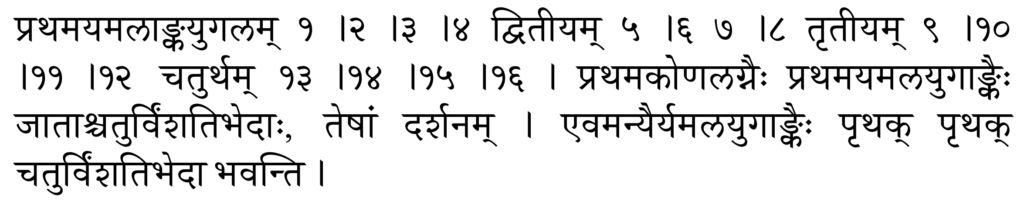
| prathamayamalā\dot{n}kayugalam 1|2|3|4 dvitīyam 5|6|7|8 tṛtīyam 9|10|11|12 caturtham 13|14|15|16\vert prathamakoṇalagnaiḥ prathamayamalayugā\dot{n}kaiḥ jātāścaturviṃśatibhedāḥ, teṣāṃ darśanam\vert evam anyairyamalayugā\dot{n}kaiḥ pṛthak pṛthak caturviṃśatibhedā bhavanti\vert |
In what follows, we present the algorithm to place all pairs of numbers through horse moves. This algorithm is tersely outlined by Nārāyaṇa Paṇḍita in just about one and a half verses (10–11a, Chapter 14 of Gaṇitakaumudī). Hence it calls for a bit of explanation. For this, we consider the following:
- Let M be a pandiagonal magic square with 16 cells (koṣṭhas) where the cells are denoted by: \[ M_{i,j} \ \ \ (i,j = 1,2,3,4) \]
- Let S be the arithmetic sequence (śreḍhi) with which the cells of M are to be filled. The sequence S that we choose for demonstration is: \[ S = \{ 1, 2, 3, 4, 5, 6, 7, 8, 9, 10, 11, 12, 13, 14, 15, 16 \} \]
It is clearly stated in the phrase catura\dot{n}ga-turagagatyā dvau dvauśreḍhīsamudbhavāva\dot{n} kau nyasya that we have to take pairs (dvau dvau) from this arithmetic sequence and place them in the magic square by way of positioning through a horse move, as done in a chessboard. The subsets to be considered from this set of numbers in the sequence are described by Nārāyaṇa Paṇḍita himself in his commentary, as yamalā\dot{n}kayugalam, meaning pair of pairs. Thus we have four subsets:
\[\begin{align*}
S_1 &= \{ 1, 2, 3, 4 \} , & \ \ \ S_2 &= \{ 5, 6, 7, 8 \} \\
S_3 &= \{ 9, 10, 11, 12 \} , & \ \ \ S_4 &= \{ 13, 14, 15, 16 \}
\end{align*}\]
In order to facilitate our discussion further we shall classify the horse moves into four types.
The four types of horse moves
From any given cell in a 4 \times 4 magic square, there are only four types of horse moves that are possible. Assume that an element p is positioned in the cell M_{1,1}. In order to place an element q in horse move with respect to p, the only four moves that are possible are illustrated in Figure 5. We denote them by U, D, L and R.
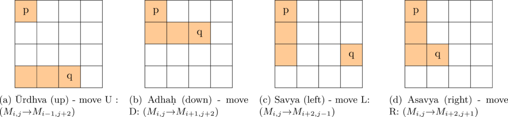
Figure 5: Four types of horse moves— U, D, L and R when p is in M1, 1.
All the twelve moves listed among the four sets H_1, H_2, H_3, and H_4 fall under one of the four types classified above. In order to describe the relative positions of certain pairs of numbers such as (2,3), (6,7), etc., Nārāyaṇa introduces two more technical terms in the above verses. We explain them in the next section.
Connotation of the phrases koṣṭhaikya and koṣṭhāntara
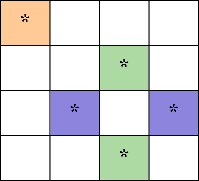
Koṣṭhaikya – placement of numbers in adjacent cells (green \rightarrow blue; or blue \rightarrow green)
Koṣṭhāntara – placement by skipping a cell in-between (green \rightarrow green; or blue \rightarrow blue)
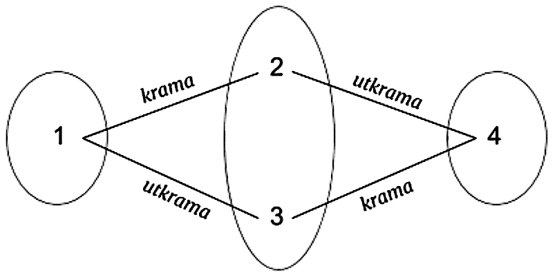
Connotation of the phrases krama and utkrama
Rule-based algorithm for placing numbers only through horse moves
For a given arithmetic series, the following rule-based algorithm tries to capture Nārāyaṇa Paṇḍita’s approach to building all possible combinations of a 4 \times 4 pandiagonal magic square.
Rules for placing pairs in \mathbf{S_1}
R.1 The first element 1 of prathamayamalā\dot{n}kayugalam S_1, is to be placed in any of the sixteen cells.
R.2 For a fixed position of 1, entry 2 can be placed by any one of the four valid horse moves – D / U / L / R, described in the previous section.
R.3 Having placed 1 and 2, 3 is also to be placed in a horse move with respect to 1 through any one of the three possible horse moves.
R.4 Having placed 1, 2 and 3, 4 is placed such that it is in a horse move from both 2 and 3. There is only one such position for any given placement of 1, 2 and 3.6
Rules for placing pairs in \mathbf{S_2, S_3 } and \mathbf{S_4}
R.5 Having placed all elements in S_1, 5 is placed such that it is always in a horse move from 1. There are only two possible ways to place 5, since 2 and 3 are already positioned through horse moves from 1. Either of them can be chosen.
R.6 All the numbers within each of the yamalā\dot{n}kayugalams in S_2, S_3 and S_4 get placed by choosing the same set of horse moves chosen for the pairs in prathama-yamalā\dot{n}ka-yugalam S_1, with the only condition that if a cell in which the subsequent number is to be placed is already filled, then the horse moves get reversed. The equivalent pairs of horse moves are presented below where the same type of horse moves will be retained. In the case of reversing a horse move, U will become D and vice versa, and L will become R and vice versa.
R.7 Having placed elements in S_1 and S_2, 9 is placed in the only horse move position that is available from 1.
R.8 Having placed elements in S_1, S_2 and S_3, 13 is placed in the only horse move position that is available from 9.7
Total possible pandiagonal magic squares
Based on the aforesaid rules, it can be observed that:
- Having fixed a position for 1, there are four possible moves for placing 2. Thus the pair (1,2) can have four different configurations.
- For a fixed position of 1, there are three possible moves for placing 3.
- It becomes evident that there will remain only one position for placing 4 in accordance with the rule R.4.
Thus at this stage, we see that there are totally 4 \times 3 = 12 possible configurations.
- For a given arrangement of 1, 2, 3, and 4, only two possible positions are available for 5 satisfying the aforesaid rule R.5. We then see that there are totally 12 \times 2 = 24 possible configurations.
- Once the numbers 1, 2, 3, 4, and 5 are fixed, the rest of the square has only a unique solution for being a pandiagonal magic square.
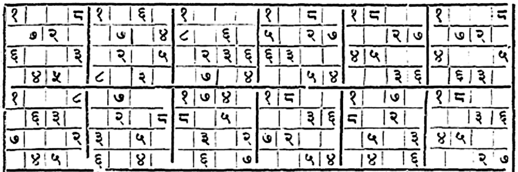
The twenty-four possible combinations for placing the numbers 1, 2, 3, 4, and 5 by placing 1 at M_{1, 1} are shown in the figure.
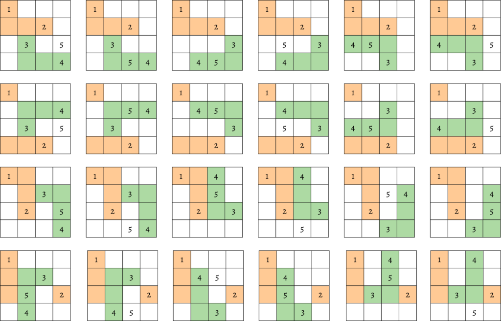
As the number 1 itself can occupy any of the sixteen cells of M, the total number of pandiagonal magic squares is 16 \times 24 = 384, as stated by Nārāyaṇa Paṇḍita. Owing to the fact that positions of all other numbers (6, 7, …, 16) get fixed once the first five are fixed, there are only 384 pandiagonal magic squares possible out of the 7,040 possible normal magic squares of order 4. This is a highly nuanced algorithm presented in Gaṇitakaumudī that doesn’t seem to have parallels elsewhere in the mathematical literature of those times, and even centuries later.
Conclusion
We have tried to set the historical context, and present an overview of the mathematical content in the monumental treatise Gaṇitakaumudī of Nārāyaṇa Paṇḍita in this article. The fourteenth century work is the largest among the extant texts in arithmetic, engaging in a lively exposition of a variety of topics, and vividly illustrating the sophistication achieved in the development of mathematics in India around that time.
Using his novel idea of the third diagonal, Nārāyaṇa Paṇḍita meticulously went through evolving possibilities and discovered several connected relations. The area, circumradius, altitude, segments of diagonals, segments of altitudes and the proportion of areas of the triangles within the quadrilateral are all relations that are not to be found elsewhere, including prominent texts such as Līlāvatī.
The turagagati method of constructing 4 \times 4 pandiagonal magic squares employing only horse moves is an algorithm that distinguishes itself for its simplicity and optimized set of rules. An interesting facet of this algorithm is that the pair of pairs can be built from the same series by a different numerical sequence as well.
For original mathematical ideation, elegant design of algorithms, as well as a systematic presentation of various topics, this work deserves much admiration. While the Līlāvatī is much acclaimed for its blend of poetry and mathematics, the hallmark of Gaṇitakaumudī is its structured, elaborate, thorough and exhaustive presentation. The grand work Gaṇitakaumudī of Nārāyaṇa Paṇḍita leaves little doubt that he is in the same league as Āryabhaṭa, Brahmagupta, Bhāskarācārya and others in the hall of fame of ancient Indian mathematicians.
Acknowledgement: The authors of the paper are deeply indebted to IIT Gandhinagar for the generous financial support extended by way of providing fellowship to the research scholars undertaking the study of the text Ganitakaumudi through the HoMI (History of Mathematics in India) Project. \blacksquare
References
- [1] V.G. Apte, Līlāvatī – Part 1, Anandashram, 1937.
- [2] Colebrooke and H.C. Banerji, Līlāvatī, Kitab Mahal, Allahabad, 1967.
- [3] K.S. Shukla (revised). B. Datta and A.N. Singh, Magic squares in India, Indian Journal of History of Science, 27(1), 51–120, 1992.
- [4] R.C. Gupta, Early Pandiagonal Magic squares in India, Bulletin of Kerala Mathematics Association, 2, 25–44, 2005.
- [5] T. Hayashi, Two Benares Manuscripts of Nārāyaṇa Paṇḍita’s Bījagaṇitāvataṃsa (Bījagaṇitāvataṃsa part II). Studies in the History of the Exact Sciences in Honour of David Pingree (Edited by Charles Burnett [et al.]) Brill 386–496, 2004.
- [6] T. Kusuba, Combinatorics and Magic Squares in India. A Study of Nārāyaṇa Paṇḍita’s Gaṇitakaumudī, Chaps. 13–14, Ph.D thesis (unpublished), Brown University, 1993.
- [7] D.N. Lehmer, A complete census of 4 × 4 magic squares, Bulletin of the American Mathematical Society, 39(10), 764 – 767, 1933.
- [8] Padmākara Dvivedī, The Gaṇita Kaumudī (Part I), The Princess of Wales Saraswati Bhavana Texts, 1936.
- [9] Padmākara Dvivedī, The Gaṇita Kaumudī (PartII), The Princess of Wales Saraswati Bhavana Texts, 1942.
- [10] Paramanand Singh, A Critical Study of the Contributions of Nārāyaṇa Paṇḍita to Hindu Mathematics, Ph.D. Thesis (unpublished), Bihar Univ., 1978.
- [11] Paramanand Singh, The Gaṇita Kaumudī of Nārāyaṇa Paṇḍita, Gaṇita Bhāratī, 20 (1-4), 25–82, 1998.
- [12] Paramanand Singh, The Gaṇita Kaumudī of Nārāyaṇa Paṇḍita, Chapter IV, Gaṇita Bhāratī, 21(1-4), 10–73, 1999.
- [13] Paramanand Singh, The Gaṇita Kaumudī of Nārāyaṇa Paṇḍita, Chapter XIV Gaṇita Bhāratī, 24(1-4), 35–98, 2002.
- [14] K.V. Sarma, K. Ramasubramanian, M. D. Srinivas, and M. S. Sriram, Gaṇita-yukti-bhāṣā, volume 1, Springer, 2009.
- [15] T.A. Sarasvati Amma, Geometry in Ancient and Medieval India, Motilal Banarsidass Publishers Private Limited, 1999.
- [16] J. Sesiano, Magic Squares, Springer International Publishing, 2019.
- [17] K.S. Shukla, Nārāyaṇa Paṇḍita’s Bījagaṇitāvataṃsa (Part I), Akhila Bharatiya Sanskrit Parishad, 1970.
Footnotes
- The word paripāṭi or simply pāṭī refers to a method or approach taken to accomplish a certain end. In the context of mathematics, it refers to the systematic approach taken to do a variety of fundamental arithmetic operations such as addition, subtraction, multiplication and division. Thus the mathematics or science associated with these operations is called pāṭīgaṇita. ↩
- One full cycle of the moon, divided into two parts, the waxing half and the waning half, is referred to in the Indian calendar as Śukla pakṣa and Kṛṣṇa pakṣa. ↩
- The calculation of actual time period is more complex as it involves knowing the instantaneous velocities of the sun and the moon. ↩
- Equi-dichastic is a quadrilateral where two pairs of two sides are equal. It could be a kite or a rectangle. ↩
- The word ūrdhva generally means above. Thus this phrase employed by Nārāyaṇa is indicative of the procedure that had been adopted to find the sum of a sequence of numbers in those periods [i.e., counting begins from the bottom row, upwards]. Or else, the term ūrdhva can also be taken as a upalakṣaṇa for adhaḥ, if we start finding the sum from the top. That is, the phrase ūrdhvasthānāṃ is understood as ūrdhvādhaḥsthānāṃ. ↩
- To quickly position 4, the following equivalent rule can be applied. Alternative rule to R4: If the relative positions of 2 and 3 placed by horse moves is a koṣṭhaikya then the type of the horse move (3,4) is the same as that of the horse move (1,2). If the relative positions of 2 and 3 are in koṣṭhāntara, then the type of the horse move (3,4) is same as that of the horse move (1,3). ↩
- Similar to R4, in order to quickly position 13 the following equivalent rule can be applied. Alternative rule to R8: If the relative positions of 5 and 9 placed by horse moves is a koṣṭhaikya then the type of the horse move (9,13) is the same as that of the horse move (1,5). If the relative positions of 5 and 9 are in koṣṭhāntara, then the type of the horse move (9,13) is the same as that of the horse move (1,9). ↩