
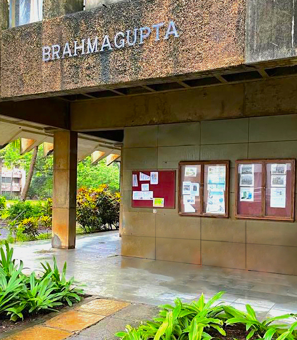
Brahmagupta (628 CE) takes up the much harder problem of finding positive integer solutions to the quadratic indeterminate equation Dx^2+1=y^2 for a fixed positive integer D. In this part, we shall revisit Brahmagupta’s composition law bhāvanā and its applications to the problem of finding integer solutions of the equation Dx^2+1=y^2. In the next part, we shall discuss further applications.
The legacy of Brahmagupta’s bhāvanā has inspired the name of this magazine; the inner front cover page of every issue contains a write-up on the concept and the term bhāvanā.
The Varga-prakṛti: An Introduction
Suppose D is a positive integer which is not a perfect square. Then we know that \sqrt{D} is an irrational number, i.e., there do not exist positive integers x,y such that \sqrt{D}=\frac{y}{x}, i.e., there do not exist integer solutions of the equation Dx^2=y^2.
But we strive to find good and convenient rational approximations to irrational numbers; for instance, we often consider the rational approximation \frac{22}{7} for \pi. How to obtain a good rational approximation \sqrt{D} \approx\frac{y}{x}? A natural approach would be to find a square x^2 whose product with the given non-square D would again become a square y^2 after adding a small integer z, preferably 1. And indeed, in ancient Indian mathematics, any equation of the type
\[\large\begin{equation}\label{z}
Dx^2+z=y^2
\end{equation}\](D a fixed positive integer) is called varga-prakṛti (square-nature), a suggestive terminology. The coefficient D is termed as guṇaka (multiplier or qualifier) or prakṛti (nature or type), while the quantity z is called kṣepa, prakṣepa or prakṣepaka (additive or interpolator). The (integer) solutions corresponding to x and y are defined by Brahmagupta as ādya-mūla (initial or first root) and antya-mūla (final or second root) respectively; later writers sometimes term them as kaniṣṭha-pada (junior or lesser root) and jyeṣṭha-pada (senior or greater root) respectively.
The central goal is to arrive at integer solutions to the special equation
\[\large\begin{equation}\label{1}
Dx^2+1=y^2,
\end{equation}\]which may be thought of as being among the closest possible modifications of Dx^2=y^2. Any solution (x,y) to the equation (2) can then be expected to yield a good rational approximation \frac{y}{x} to \sqrt{D}.
Note that the equation (1) poses a serious challenge only when D is a non-square positive integer. For, if D<0, then, for a fixed integer z, it is easy to see that there are at most finitely many integer solutions of the equation (1). Again, if D is a perfect square and z a fixed nonzero integer, then, by factoring y^2-Dx^2, it is easy to see that (1) has only finitely many integer solutions and one can easily determine them. For instance, (0, \pm 1) are the only integer solutions of (2) when D is a perfect square.1 Thus one is interested only in those values of D which are positive integers but not perfect squares. We shall later see that, in this case, (2) has infinitely many solutions in positive integers.
Now, for small values of D, a solution of (2) can be found by inspection. For instance, when D=2, one can readily find an integer solution of 2x^2+1=y^2, namely, (x,y)=(2,3). But this is misleadingly simple. For, when D=61, the smallest positive integer solution of
\[\large\begin{equation}
61x^2+1=y^2
\end{equation}\]is
\[\large\begin{equation}
(x,y)=(226153980, 1766319049)
\end{equation}\]indicating the unexpected intricacy of the problem. In contrast to this case, for D=60, the minimum positive integer solution of 60x^2+1=y^2 is (x,y)=(4,31).
In the preface of his famous book “History of the Theory of Numbers” Vol II (1920), L.E. Dickson emphasizes the difficulty of finding rational or integer solutions of quadratic equations in two variables whose loci are conics ([9], p. iii):
whose coordinates are rational and a greater difficulty
to pick out those points whose coordinates are integral.
The Varga-prakṛti: A Brief History
Brahmagupta’s pioneering work on the varga-prakṛti
The first major breakthrough to the problem of solving Dx^2+1=y^2 is achieved by Brahmagupta in 628 CE when he comes up with his master-stroke: his composition law bhāvanā on the solution space of the more general equation Dx^2+z=y^2. The precise statement will be recalled in the next section in modern language.
Brahmagupta applies his composition rule to generate an infinite number of integer solutions from a given integer solution of Dx^2+1=y^2 and also shows how to arrive at an integer solution in a wide variety of cases (e.g., D=83 or D=92).
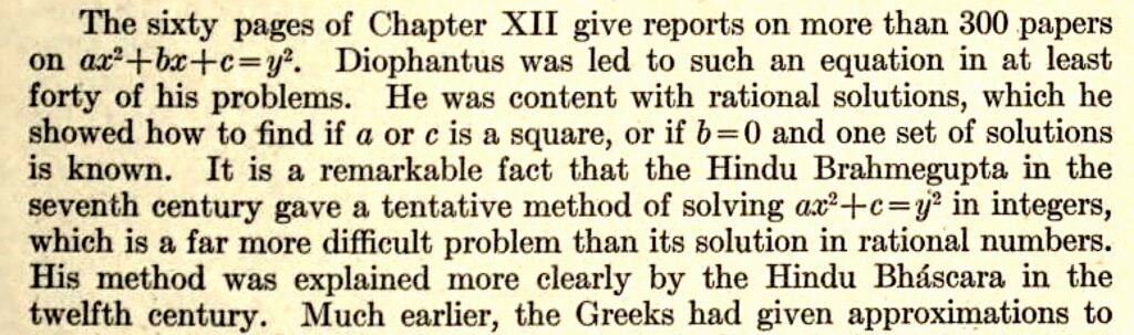
In the preface of his book [9], Dickson makes a considerable mention of Indian contributions to the study of indeterminate equations. He makes a special mention of Brahmagupta’s work ([9], p. xi):
in the seventh century gave a tentative method of
solving ax^2+c=y^2 in integers, which is a far more
difficult problem than its solution in rational numbers.
The reader should note that such genuine words of appreciation however miss the real greatness of Brahmagupta’s work on indeterminate equations — his manifestation of the very principle of `composition’ (or `binary operation’) in mathematics, for the first time in known history. The idea of the composition of two objects of the same type to produce a third object of the same type is the quintessence of modern abstract algebra and pervades many branches of modern mathematics.
Brahmagupta’s methods, once stated, are easy to understand and implement. To have a richer appreciation of these techniques, young readers could first spend some time attempting to devise their own methods for finding integer solutions of equation (2) for special values of D. Before going to the next section, the students could at least try the simple exercise:
Exercise 1. Consider 11x^2+1=y^2. By trial-and-error, if not by ready inspection, one can easily arrive at the smallest positive integer solution (3, 10). Find a larger solution.
Further development on the varga-prakṛti after Brahmagupta
While Brahmagupta gives a partial solution to the problem of finding integer solutions of (2), later Indian algebraists discover the complete integer solution by a cyclic method called cakravāla (cakra: wheel or disc) in ancient India. The earliest description of the cakravāla algorithm, known to us so far, is due to the mathematician Jayadeva; his verses on the cakravāla algorithm have been quoted in the text Sundarī of Udayadivākara composed in 1073 CE. Nothing is known so far about the mathematician Jayadeva, except that he lived sometime between the seventh century (after Brahmagupta) and the eleventh century (before Udayadivākara). He is not to be confused with the Vaiṣṇava poet Jayadeva of the twelfth century who composed Gīta-Govinda. Udayadivākara’s text Sundarī, containing Jayadava’s verses, was discovered only in 1954 by K.S. Shukla.
The famous astronomer-mathematician Bhāskara II (1150 CE), who is also referred to as Bhāskarācārya, describes the cakravāla and illustrates it with difficult numerical cases like D=61 and D=67. The mathematician Nārāyaṇa (c. 1350 CE) too discusses the cakravāla and illustrates the method with the cases D=97 and D=103, and shows how to use the solutions to give rational approximations to \sqrt{D}. We plan to discuss the three descriptions of the cakravāla algorithm in a subsequent part of this series.
Besides the equations ay-bx=c and Dx^2+z=y^2, several other indeterminate and simultaneous indeterminate equations occur in the treatises of some of the above mathematicians, especially Bhāskara II. The Indian results on varga-prakṛti and other indeterminate equations have been discussed by Datta-Singh in [8]; K.S. Shukla has presented the results of Jayadeva on varga-prakṛti in [15].
The equation Dx^2+1=y^2 in modern Europe
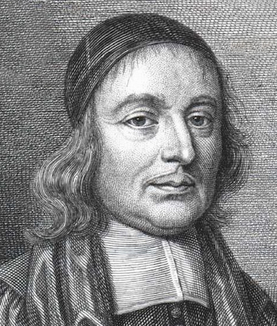
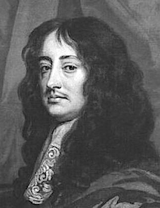
Pierre de Fermat (1601–65), who is regarded as the father of modern number theory, tries to create enthusiasm for the subject among his contemporary mathematicians like John Wallis (1616–1703) and Lord William Brouncker (1620–84) of England, B. Frenicle de Bessy (c. 1612–75) of France and F. van Schooten3 (1615–60) of the Netherlands.
Now arithmetic has, so to speak, a special domain of its own, the theory of integral numbers. This was only lightly touched upon by Euclid in his Elements, and was not sufficiently studied by those who followed him […]; arithmeticians have therefore now to develop it or restore it.
To arithmeticians therefore, by way of lighting up the road to be followed, I propose the following theorem to be proved or problem to be solved. If they succeed in discovering the proof or solution, they will admit that questions of this kind are not inferior to the more celebrated questions in geometry in respect of beauty, difficulty or method of proof.
Given any number whatever which is not a square, there are also given an infinite number of squares such that, if the square is multiplied into the given number and unity is added to the product, the result is a square.
Regarding Fermat’s challenge, André Weil remarks ([18], pp. 81–82):
A general method for solving Fermat’s problem is discovered by Brouncker in 1657. In response to a challenge posed by Frenicle, Brouncker is able to use his method to find the (smallest) solution x=1819380158564160,\quad y=32188120829134849 to the equation 313x^2+1=y^2 which he claims has taken him only “an hour or two”.5
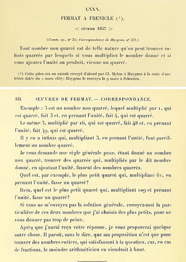
During 1657–58, there have been exchanges of letters among mathematicians like Frenicle, Brouncker and Wallis on Fermat’s problem; these letters are published by Wallis in Commercium Epistolicum (1658). Fermat asserts that he can prove by his method of “descent” that the equation Dx^2+1=y^2 has infinitely many integer solutions (when D is a positive integer which is not a perfect square), but the proof has not been found in any of his writings.
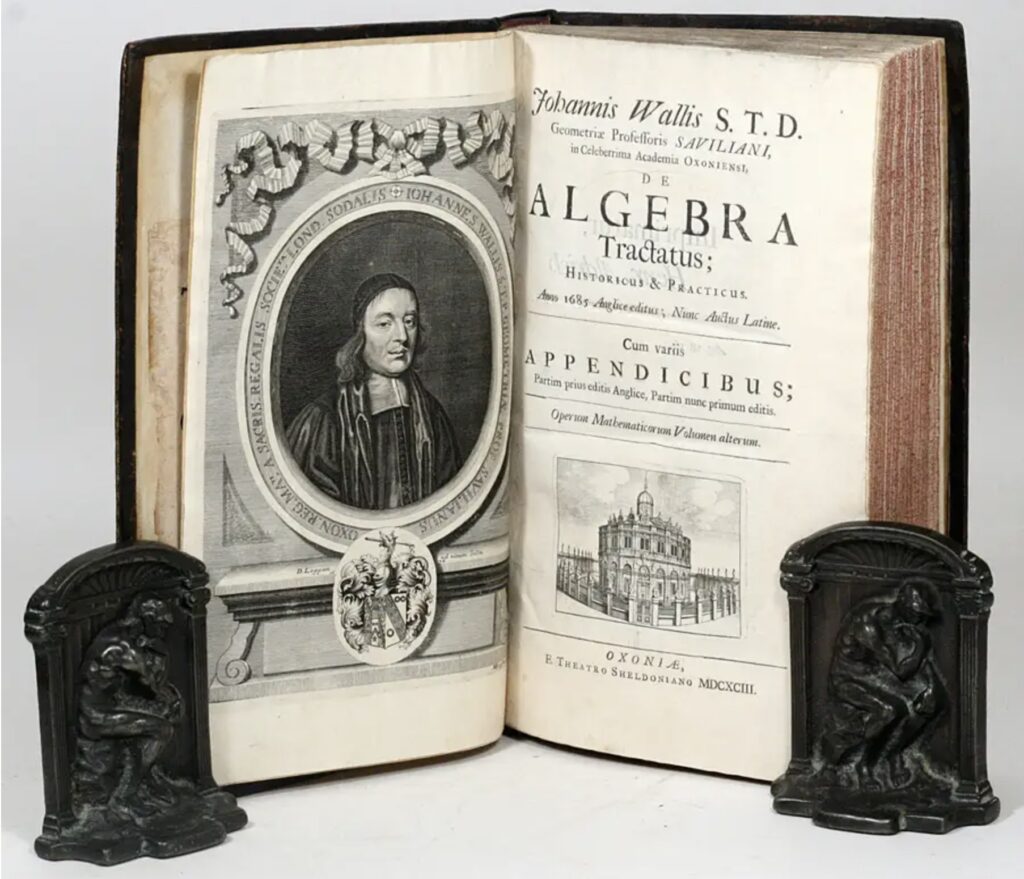
In 1685, Wallis publishes his monumental work A treatise of algebra both historical and practical (in short, Algebra) comprising 100 chapters. Chapter 98 of this treatise is devoted to Fermat’s problem and is based on the correspondence published in Commercium Epistolicum. Brouncker’s method for solving the equation Dx^2+1=y^2 is described in this chapter in a standard form. An enlarged second edition of the treatise Algebra is published as the second volume of Wallis’ Opera Mathematica (1693). Wallis attempts to prove that Dx^2+1=y^2 always has a positive integer solution, but uses an incorrect result ([9], p. 354).
Fermat’s problem is again taken up in the next century by the two greatest figures of eighteenth-century mathematics: L. Euler (1707–83) and J.L. Lagrange (1736–1813). Euler becomes interested in the problem from around 1730 and Lagrange takes it up around 1768. They develop the theory of continued fractions, investigate the problem in the framework of this theory and establish that if D is not a perfect square, then \sqrt{D} has an infinite but periodic continued fraction expansion, and all solutions (p,q) to the equation Dx^2+1=y^2 are given by certain convergents \frac{q_n}{p_n} of the expansion.6 Moreover, there exists a positive integer solution (x_1,y_1) of Dx^2+1=y^2 (called the fundamental solution) such that all positive integer solutions are given by (x_n, y_n) where x_n, y_n are defined by the relation y_n + \sqrt{D} x_n = (y_1 + \sqrt{D} x_1)^n. While the initial discoveries are made by Euler, it is Lagrange who first publishes formal proofs of all these results during 1768–69. He includes them in his Additions to Euler’s Elements of algebra (composed in 1771, published in 1773). The precise historical details are given in ([18], p. 183; pp. 229–233).7
The label “Pell’s equation”
Selberg mentions in an interview8 that André Weil once said that if something in mathematics gets attached to the name of a person, then the person in question usually has very little to do with it.
The equation Dx^2+1=y^2 gets attributed to the English mathematician John Pell (c. 1611–85) by Euler although there is no evidence that John Pell had seriously investigated the equation. Euler’s confusion could have been created through a cursory reading of Wallis’ Algebra, a large part of which is devoted to the work of five English mathematicians: Oughtred, Harriot, Pell, Newton and Wallis himself. In any case, the name “Pell’s equation” stuck. As Weil puts it ([18], p. 174):
Since Brahmagupta is the first known mathematician to investigate this important equation in a general framework, the equation Dx^2+1=y^2 is nowadays being gradually renamed as the Brahmagupta–Pell equation.
Some ancient problems involving Dx^2 \pm 1=y^2
Some of the rational approximations to \sqrt{D}, which appear in (late Vedic) Indian and Greek texts, implicitly involve equations of the type Dx^2+1=y^2. In the Śulba-sūtras (c. 800 BCE), the most ancient extant mathematics treatises, \frac{7}{5}, \frac{17}{12}, \frac{577}{408} have been used as approximations for \sqrt{2} ([7], p. 202); [9], p. 341). These three fractions may be interpreted as arising out of solutions of 2x^2 \pm 1=y^2; for
2 \times 5^2-1=7^2, 2 \times 12^2+1=17^2, 2 \times 408^2+1=577^2.In fact, they are respectively the third, fourth and eighth convergents of the simple continued fraction expansion of \sqrt{2}.
Archimedes (287–212 BCE) gives the approximations \frac{265}{153} and \frac{1351}{780} for \sqrt{3}. In his commentary on the work of Archimedes, Eutocius (c. 480–540 CE) mentions the relations 265^2-3 \times 153^2=-2 and 1351^2-3 \times 780^2=1 as a verification of the validity of the approximations ([18], p. 16).
In 1773, G.E. Lessing discovers an ancient Greek epigram which states a problem (known as the “Cattle Problem”) which is believed to have been communicated by Archimedes to Eratosthenes for the mathematicians of Alexandria. In this problem, one is required to find eight integers (number of bulls and cows each of four colours) satisfying nine conditions linear and quadratic. After some algebraic manipulations, the cattle problem reduces to the problem of finding a positive integer solution to Dx^2+1=y^2 where D=4729494. There is no evidence that Archimedes had made this connection and it is thought extremely unlikely that either Archimedes or any of his contemporaries had actually solved the cattle problem. The problem is first solved by A. Amthor (1880 CE); the smallest value of one of the variables in the cattle problem is a number having 206545 digits (cf. [9], pp. 342–345; [14] for further details).
Legacy of “Pell’s equation”
The study of indeterminate equations, especially the study of the so-called “Pell’s equation”, has played an important role in the evolution of classical algebra in ancient India and later in modern Europe.9
Pell’s equation has had applications throughout history. As we shall see, large integer solutions of Dx^2+1=y^2 have been used in ancient India to yield good rational approximations to \sqrt{D}. The solutions of the equation yield units in the domain of “integers of the quadratic field \mathbb{Q}(\sqrt{D})”. The equation is also closely related to the study of “binary quadratic forms”.
The solution of Pell’s equation is the main step in the solution of the general quadratic Diophantine equation in two variables. It also plays a role in the solution (1970) of Hilbert’s 10th problem on the non-existence of an algorithm for solving arbitrary Diophantine equations.
Pell’s equation continues to fascinate mathematicians even today. Research papers and articles are being published on it in various contexts. The algorithmic efficiency of various methods is discussed in the article [14] of H.W. Lenstra. There is even an expository book [2] focusing exclusively on the topic. The author E.J. Barbeau remarks in the Preface:
Efficient generation of solutions of the equation is a very active area of research in algorithmic number theory and computer science. While there does not exist any polynomial-time classical algorithm for solving Pell’s equation, S. Hallgren has exhibited a polynomial-time quantum algorithm for the equation.10 As Lenstra remarks ([14], p. 192):
Brahmagupta’s bhāvanā
Suppose that a,b are natural numbers such that Da^2+1=b^2, i.e., b^2-Da^2=1. Squaring both sides, we have, (b^2+Da^2)^2-D(2ba)^2=1. Thus from the solution (a,b) of Dx^2+1=y^2, we produce a bigger solution (2ab, b^2+Da^2). We can continue this process to generate infinitely many distinct solutions.
In Exercise 1, from the solution (3, 10) of 11x^2+1=y^2, one gets a larger solution (2 \times 3 \times 10, 10^2+11 \times 3^2)=(60, 199). One can verify that 11 \times {60}^2+1=39601={199}^2.
Brahmagupta’s bhāvanā makes a profound generalisation, with enormous and far-reaching implications, of the above simple observation. We plan to present his Sanskrit verses, with word-by-word translations, in a subsequent issue. Brahmagupta’s main principle, the bhāvanā can be formulated, in modern language and notation, as follows:
Theorem 1.[Brahmagupta’s bhāvanā] The solution space of the equation Dx^2+z=y^2 admits the binary operations\[\large\begin{align*}(x_1,y_1,z_1) \odot (x_2,y_2,z_2)\qquad\qquad\qquad\qquad\\
= (x_1y_2 + x_2y_1, Dx_1x_2 + y_1y_2, z_1z_2),\end{align*}\]and\[\large\begin{align*}(x_1,y_1,z_1) \star (x_2,y_2,z_2)\qquad\qquad\qquad\qquad\\
= (x_1y_2 – x_2y_1, Dx_1x_2 – y_1y_2, z_1z_2).\end{align*}\]In other words, if (x_1,y_1,z_1) and (x_2,y_2,z_2) are solutions of Dx^2+z=y^2, then so are (x_1y_2+x_2y_1, Dx_1x_2+y_1y_2, z_1z_2) and (x_1y_2-x_2y_1, Dx_1x_2-y_1y_2, z_1z_2).
Theorem 1 has also been stated in verse form by Ācārya Jayadeva, Bhāskara II (1150 CE), Nārāyaṇa (1350 CE), Jñanarāja (1503 CE) and Kamalākara (1658 CE). We quote below the lucid presentation of Bhāskara II:
[Consider] the desired lesser root [x]. Its square, multiplied by prakṛti [D], is added or subtracted by some quantity [c] such that it [the sum or difference Dx^2 \pm c] gives a [integer] square root. The interpolator [m= \pm c], positive or negative, is called the kṣepa; the square root [y] is called the greater root.
Set down successively the lesser root [x_1], the greater root [y_1] and the interpolator [m_1]. Place under them, the same or another [triple x_2, y_2, m_2], in the same order. From them, by repeated applications of the bhāvanā, numerous roots can be sought. Therefore, the bhāvanā is being expounded.
[Consider] the two cross-products of the two greater and the two lesser roots. The sum [x_1y_2+x_2y_1] of the two cross-products is a lesser root. Add the product of the two [original] lesser roots multiplied by the prakṛti [D] to the product of the two greater roots. The sum [Dx_1x_2+y_1y_2] will be a greater root. The product of the two [previous] interpolators will be the [new] interpolator.
Again the difference between the two cross-products is a lesser root. The difference between the product of the two [original] lesser roots multiplied by the prakṛti and the product of the two greater roots will be a greater root. Here also, the interpolator is the product of the two [previous] interpolators.
A Proof
Brahmagupta's result (Theorem 1), once stated, is not difficult to prove. Proofs of such results are not to be expected in the original treatises, where even the statements of main results are usually terse. They were communicated orally and sometimes recorded in the later works.
A proof of Theorem 1 is described by Kṛṣṇa Daivajña in his treatise Bījapallava (1548).11 In this proof, one can see the similarity with the profound idea of “completing the square” in the theory of quadratic equations that we had discussed in ([12], pp. 59–62), an idea regarded very highly by Late Shreeram Abhyankar. We present it below.
Proof: We are given:
\[\large\begin{equation}\label{given1}
D{x_1}^2+z_1={y_1}^2
\end{equation}\]and
\[\large\begin{equation}\label{given2}
D{x_2}^2+z_2={y_2}^2
\end{equation}\]Multiplying (5) by {y_2}^2, we get
D{x_1}^2{y_2}^2+z_1{y_2}^2={y_1}^2{y_2}^2.Hence, using (6), we get
D{x_1}^2{y_2}^2+ z_1 (D{x_2}^2+z_2)={y_1}^2{y_2}^2,that is,
D{x_1}^2{y_2}^2+ z_1D{x_2}^2+z_1z_2={y_1}^2{y_2}^2.Hence, using (5), we get
D{x_1}^2{y_2}^2+ ({y_1}^2-D{x_1}^2)D{x_2}^2+z_1z_2={y_1}^2{y_2}^2,that is,
D{x_1}^2{y_2}^2+ D{x_2}^2{y_1}^2+z_1z_2={y_1}^2{y_2}^2+D^2{x_1}^2{x_2}^2.Adding \pm 2Dx_1x_2y_1y_2 to both sides for “completing the squares”, we have
Realization of the importance
For brevity, we shall adopt a notation suggested by Weil ([18], p. 21). For a given positive integer D, (p,q;m) will denote a triple of numbers satisfying Dp^2+m=q^2. Thus Theorem 1 states:
(p, q; m)\odot(r, s; n)=(ps + qr, D pr + qs ; mn),and
(p, q; m)\star(r, s; n)=(ps - qr, D pr - qs ; mn).We shall use the notation (p,q;m)^n to denote (p,q;m)\odot (p,q;m) \cdots \odot (p,q;m), n times.
Ancient Indian algebraists demonstrate a realization of the importance of the laws and name them by the special technical term bhāvanā (composition) – the formula obtained by taking the positive sign (i.e., the operation \odot) is called the samāsa-bhāvanā 12 or yoga-bhāvanā (additive composition) and the one obtained by taking the negative sign (i.e., the operation \star) is called the viśeṣa-bhāvanā or antara-bhāvanā (subtractive composition). In the special case of equal roots and interpolators, the rule is called tulya-bhāvanā (composition of equals); the general case is called atulya-bhāvanā (composition of unequals).13 Unless otherwise stated, the term bhāvanā usually refers to the additive composition samāsa-bhāvanā.
In a commentary on Brāhma-Sphuṭa-Siddhānta (see [5], pp. 363–364), it is repeatedly emphasised, during the exposition of Brahmagupta's verses stating Theorem 1, that the new roots (x,y,z) have been obtained from the given roots (x_1, y_1, z_1), (x_2,y_2,z_2) by composition.
Just before stating the bhāvanā formulae, Jayadeva mentions ([15], p. 5) that the bhāvanā operations pervade numerous algorithms. In the light of modern developments, Jayadeva's statement has turned out to be prophetic.
The importance attached to the bhāvanā also comes out in Bhāskara II's exposition of the concept quoted earlier, where he states:
The perception of Theorem 1 as a law of composition (i.e., in terms of an operation like \odot) comes out in the applications by Brahmagupta and others, in the version of Theorem 1 due to Bhāskara II and, above all, in the choice and use of the term bhāvanā (“composition”).
The term bhāvanā
In general, the Sanskrit word bhāvanā has several meanings including “production” and “demonstration”; in the context of mathematics, bhāvanā means “composition” or “combination”.
A similar Sanskrit word bhāvita (usual meaning: “created”, “produced”; or “future”, “to be”) is used in Indian algebra by Brahmagupta and others to denote the product of different unknown quantities. The law \odot (or \star) is perceived as a special mathematical operation involving a special multiplicative principle. In fact, Udayadivākara (1073 CE) explains bhāvanā as multiplication ([15], p. 6).
While the principal sense of bhāvanā, in the context of \odot (or \star), is that of a principle of “composition” — a sort-of generalised “product” — the term also carries the additional suggestion of being a principle of “production” (i.e., “generation”) of new roots, and of being a powerful “producer” of new results.
For a further discussion on the rich significance of the term, see ([10], pp. 14–15).
Significance of bhāvanā as binary composition
Theorem 1 defines the intricate binary operation (samāsa-bhāvanā)
(x_1,y_1;z_1) \odot (x_2,y_2;z_2) = (x_1y_2 + x_2y_1, Dx_1x_2 + y_1y_2, z_1z_2)on the set S=\{(x,y,z) \in {\mathbb Z} \times {\mathbb Z} \times {\mathbb Z} | Dx^2+z=y^2 \} where \mathbb{Z} denotes the set of integers. This sophisticated idea of constructing a binary composition on an abstractly defined unknown set is the quintessence of modern “abstract algebra”.
The idea occurs in Brahmagupta's work in a fluid-like amorphous form, not yet crystallised into a precise set-theoretic framework. Brahmagupta does not present the collection S as a single entity. However, Brahmagupta envisages the key ingredient of a modern abstract structure: binary composition. If one excludes the four elementary arithmetic operations on usual numbers, the bhāvanā is perhaps the first conscious construction of a binary composition.
Further, the binary operation, involving two integral triples of unknown roots, is not only intricate, it involves ideas far ahead of the times. Basic symbolic computations with unknown roots, treating them as if they are known quantities, is a fairly modern approach that would emerge during the investigations on the general polynomial in one unknown, during the late eighteenth century.
The discovery of an algebraic structure, such as Brahmagupta's composition law, on a set of significance, is now an important theme in certain frontier areas of modern mathematics research. For instance, the “addition law” on the points of an elliptic curve14 is a basic tool in the study of the curve.
As elaborated in ([12], pp. 65–66) it is only at the research level that some students of mathematics come across the idea of constructing a suitable composition law on an important set, i.e., to impart an abstract structure on the set, for a deeper study of the set; and that too if the students specialize in certain directions. And such an idea occurs in the work of a creator of classical algebra!
Some applications of bhāvanā in India
In a lecture on as broad a topic as Mathematics as a basic science, Michael Atiyah15 observed:16
Brahmagupta's presentation of the results on varga-prakṛti resembles a typical modern arrangement where one first develops the fundamental theory or principle that emerges out of the investigations into a problem, and then records the solution to the original problem(s) as one application of the basic theory. Thus, after announcing atha varga prakṛtiḥ, Brahmagupta immediately states Theorem 1 – the cornerstone of the section on varga-prakṛti – in Verses 64–65 of ([3], Ch. 18). This is followed by a few general results on the varga-prakṛti which are useful offshoots of Theorem 1: construction of infinitely many rational solutions of Dx^2+1=y^2 (Verse 65), generation of infinitely many integer solutions of Dx^2 +m=y^2 from a given one (Verse 66), derivation of solutions of Dx^2+1=y^2 from solutions of Dx^2 \pm 4=y^2 (Verses 67–68), etc. The results are then illustrated by several concrete numerical examples. We first mention a few applications and examples of Brahmagupta himself and then a few later applications.
Application 1: Rational solutions of Dx^2+1=y^2
Immediately after stating their respective verses describing Theorem 1, Brahmagupta, Jayadeva ([15], p. 8) and Bhāskara II ([4], p. 23) describe non-trivial rational solutions of Dx^2+1=y^2. This is actually an easy application – the full strength of Theorem 1 is not really needed. Brahmagupta's verses 64–65 in ([3], Ch. 18) contain, apart from Theorem 1, the above application through the following two immediate corollaries:
Corollary 1: [Brahmagupta] If Dp^2+m=q^2, then D(2pq)^2+m^2=(Dp^2+q^2)^2.
Corollary 2: [Brahmagupta] If (p,q) is a root of the equation Dx^2 \pm c=y^2, then (\frac{2pq}{c}, \frac{Dp^2+q^2}{c}) is a root of Dx^2 + 1=y^2.
Corollary 1 can be seen to hold directly, since the given hypothesis implies that
m^2=(q^2-Dp^2)^2=(Dp^2+q^2)^2-D(2pq)^2. and Corollary 2 follows.
To get a rational solution of Dx^2+1=y^2, one can choose a positive integer p (for instance, p=1) and a positive integer q such that q^2>Dp^2, set m:=q^2-Dp^2 to get Dp^2+m=q^2 and then apply Corollary 2.
Note that Brahmagupta simply makes a terse statement amounting to Corollary 2but does not give any easy explanation as to how to obtain some integer-triple (p,q; m). As highlighted earlier in this series ([11], p. 57), brevity is a general feature of the treatises of earlier greats like Āryabhaṭa (499 CE) and Brahmagupta (628 CE) who give broad hints and not complete details; we had also pointed out that, like the ancient Indian masters, many modern mathematicians too engage in terse expositions.
But as the history of algebra from the 1870s will testify, clarity of exposition can sometimes do wonders for the rapid progress of a subject. In ancient Indian algebra, the terseness of Brahmagupta is balanced by the clearer accounts of later expositors. For instance, Śrīpati (1039 CE) describes the method for obtaining rational solutions as follows:
In other words, applying Brahmagupta's bhāvanā (Theorem 1) on two copies of the identity
D\cdot1^2+(q^2-D)=q^2, one gets a rational solution x=\frac{2q}{q^2 \sim D}, y=\frac{q^2+D}{q^2 \sim D} of Dx^2+1=y^2. Infinitely many roots can be obtained by varying q (also by repeated use of bhāvanā).
The above solution is also described by Bhāskara II (1150 CE), Nārāyaṇa (1350 CE) and later writers like Jñānarāja (1503 CE), Kṛṣṇa (1548) and Kamalākara (1658 CE). To quote Bhāskara II:
The application of bhāvanā on the identity
D\cdot1^2 + q^2-D = q^2 to obtain rational solutions may appear to be a relatively minor feat in the history of Indian algebra. However, the brief discussion on the cakravāla in a later subsection will show that the clear formulation of the above identity, the display of the action of bhāvanā on it, and the explicit mention of division by q^2-D must have facilitated the invention of the cakravāla. We can also expect that, during actual computation, of rational solutions of Dx^2+1=y^2, there would have been a tendency to choose q so as to avoid division by large numbers. This leads to a q for which |q^2-D| is the minimum – another component of the complex cakravāla. In this connection, one is reminded of Weil's caveat ([17], p. 235):
Application 2: Generation of infinitely many roots
The general equation Dx^2+m=y^2 need not have any integer solution. For instance, 3x^2+2=y^2 does not have any integer solution since there is no integer y satisfying y^2 \equiv 2 (\mod 3).
However, when it does have an integer solution (p,q; m), and when knows a non-trivial integer solution (\alpha, \beta; 1) of Dx^2+1=y^2, Brahmagupta's verse 66 prescribes composing (p,q; m) with (\alpha, \beta; 1) (using Theorem 1) repeatedly (i.e., by considering (p,q;m) \odot (\alpha, \beta; 1)^n for n=1, 2, …), one generates infinitely many integer solutions of the equation Dx^2 +m=y^2. In particular, from one positive integer solution of Dx^2+1=y^2, one gets infinitely many.
Application 3: Integer solution of Dx^2+1=y^2 (Partial)
As a consequence of Theorem 1, Brahmagupta gives his partial solution to the original problem ([3], Ch 18, verses 67–68) in the following form:
Theorem 2: [Brahmagupta]
- If Dp^2+4=q^2, then (\frac{1}{2}p(q^2-1), \frac{1}{2}q(q^2-3)) is a solution of Dx^2+1=y^2.
- If Dp^2-4=q^2, and r= \frac{1}{2}(q^2+3)(q^2+1), then (pqr, (q^2+2)(r-1)) is a solution of Dx^2+1=y^2.
- [1] M. Atiyah, Mathematics as a basic science, Current Science Vol. 65(12), 912–917 (1993).
- [2] E.J. Barbeau, Pell's Equation, Springer (2003).
- [3] Brahmagupta, Brāhma-Sphuṭa-Siddhānta (628). The Sanskrit text, edited by R.S. Sharma, has been published by the Indian Institute of Astronomical Research (1966).
- [4] Bhāskarācārya, Bījagaṇita (1150). The Sanskrit text, edited and translated by S.K. Abhyankar, has been published by the Bhaskaracharya Pratishthana, Pune (1980).
- [5] H.T. Colebrooke, Algebra, with Arithmetic and Mensuration, from the Sanscrit of Brahmegupta and Bhascara, John Murray, London (1817).
- [6] B. Datta, Nārāyaṇa's Method for Finding Approximate Value of a Surd, Bulletin of the Calcutta Mathematical Society, Vol. 23 No. 4 (1931), p. 187–194.
- [7] B. Datta, The Science of the Sulba, University of Calcutta (1932); reprint (1991).
- [8] B. Datta and A.N. Singh, History of Hindu Mathematics: A Source Book Part II (Algebra), Motilal Banarsidass, Lahore (1935); Asia Publishing House, Bombay (1962).
- [9] L.E. Dickson, History of the Theory of Numbers Vol II, Chelsea Publishing Co. NY (1952).
- [10] A.K. Dutta, The bhāvanā in Mathematics, Bhāvanā, 1(1), 13–19 (January 2017).
- [11] A.K. Dutta, Mathematics in Ancient India Part 5: The Kuṭṭaka Algorithm, Bhāvanā, Vol. 7(1), 52–67 (January 2023).
- [12] A.K. Dutta, Mathematics in Ancient India Part 6: The Foundations of Algebra — Glimpses, Bhāvanā, Vol. 7(2), 52–68 (April 2023).
- [13] J.R. Goldman, The Queen of Mathematics: A Historically Motivated Guide to Number Theory, A.K. Peters (1997).
- [14] H.W. Lenstra, Solving the Pell Equation, Notices AMS, Vol. 49(2), pp. 182–192 (February 2002).
- [15] K.S. Shukla, Ācārya Jayadeva, The Mathematician, Gaṇita 5 (1954), pp. 1–20.
- [16] K.N. Sinha, Śrīpati: An Eleventh-Century Indian Mathematician, Historia Mathematica, 12 (1985), pp. 25–44.
- [17] André Weil, History of Mathematics: Why and How, Proceedings of the International Congress of Mathematicians, Helsinki 1978 Vol 1 (ed. O. Lehto), Helsinki (1980), pp. 227–236.
- [18] André Weil, Number Theory: An approach through history from Hammurapi to Legendre, Birkhäuser (1984).
- Editor’s note: See page 22, right column of the article `Timeless Geniuses, Celestial Clocks and Continued Fractions’ by Sudhir Rao in the inaugural January 2017 issue of Bhāvanā. ↩
- To give an analogy, the result on solvability by radicals of a polynomial is merely one application of the Fundamental Theorem of Galois Theory, relating subfields of a Galois extension L|_k with subgroups of the automorphism group G(L|_k), which is a central theorem in algebra with profound impact in different areas of mathematics. ↩
- A Dutch mathematician who is most famous for popularizing the cartesian geometry of Descartes. ↩
- Here “arithmetic” refers to “higher arithmetic”, i.e., number theory, the study of abstract properties of numbers. In Greece, usual computational arithmetic was called “logistic” while the term “arithmetic” meant number theory. ↩
- J.J. O'Connor and E.F. Robertson, Pell's equation ↩
- We plan to discuss the connection of the equation Dx^2+1=y^2 with the theory of continued fractions in a subsequent part of this series. Meanwhile, readers may look at Chapters XXIV and XXXIII of the book “Higher Algebra” by Barnard and Child or Chapters XXV and XVII–XXVIII of the book “Higher Algebra” by Hall and Knight for an organised presentation of the theory of continued fractions with application to the equation Dx^2+1=y^2. A well-motivated reader-friendly account of the theory is presented in chapter 4 of [13]. Silverman's book “A Friendly Introduction to Number Theory” (Third edition) gives a beautiful account of the simple continued fraction and the solution of the equation Dx^2+1=y^2 (Chapters 30, 39 and 40). ↩
- Editor’s note: The article by Arshay Sheth in this issue of Bhāvanā carries some of these details from the perspective of the lasting impact of the study of the Brahmagupta–Pell equation. ↩
- Bulletin AMS, 45(4), October 2008, p. 621. ↩
- I.G. Bashmakova has emphasised that solving indeterminate equations was a significant part in the development of algebra in Europe; for instance, in her article Diophantine equations and the evolution of algebra in the Proceedings of the International Congress of Mathematicians (ICM), Berkeley, California (1986). ↩
- S. Hallgren, Polynomial-Time Quantum Algorithms for Pell's Equation and the Principal Ideal Problem, Jour. ACM, 54(1), 1–19 (2007). ↩
- See [8], pp. 148–149; or Bījapallava of Kṛṣṇa Daivajña by Sita Sunder Ram, Kuppuswami Sastri Research Institute (2012), pp. 74–77. ↩
- From the Vedic era, addition has been called samāsa (“putting together”) and the sum obtained samasta (“whole”, “total”, etc) – see [7], p. 226. Note that the prefix sam (together) is used like the Latin con expressing “conjunction”, “union”, etc. ↩
- See ([15], pp. 5–8; [8], pp. 146–148). ↩
- Editor’s note: An elliptic curve is a curve in the (x,y)-plane defined by a cubic equation of the form y^2=x^3 + ax + b, where a and b are constants such that 4a^3 + 27b^2 \neq 0 (this condition ensures that the curve has no cusps or self-intersections). ↩
- Michael Atiyah (1929–2019) was awarded the Fields Medal in 1966 and the Abel Prize in 2004, the two highest awards in mathematics. See the July 2017 issue for an interview of his in Bhāvanā, pp. 5–18. ↩
- See Current Science, Dec.1993, p. 913. ↩
- Verse 33 of Chapter 14 (on algebra) of the astronomy treatise Siddhāntaśekhara; quoted (in translation) in ([16], p. 40; [8], p 153, p. 150). ↩
- Verse 73 of Bījagaṇita ([4], p. 23); quoted (in translation) in ([8], p. 154). ↩
- http://www.gap-system.org/~history/HistTopics/Pell.html. ↩
The results (i) and (ii) can be obtained by considering the products (p,q;4)^3 and (p,q;4)^6 respectively and making necessary substitutions and simplifications.
For instance, for (i), using the relations (p,q;4) \odot (p,q;4)=(2pq,Dp^2+q^2;4^2) and Dp^2=q^2-4, and cancelling the common factor 4 from the consequent identity D(2pq)^2+4^2=(2q^2-4)^2, one gets the triple (pq, q^2-2;4). Next, considering the composition (p,q;4) \odot (pq, q^2-2;4) and making adjustments as above, one arrives at the triple (\frac{1}{2}p(q^2-1), \frac{1}{2}q(q^2-3);1). This is an integer triple, since p(q^2-1) and p(q^2-3) are even. This is obvious if p is even. If p is odd, then so will be q, so that q^2-1 and q^2-3 would be even.
Since (\pm 1)^2=1 and (\pm 2)^2=4, it follows that from any positive integer solution of Dx^2+m=y^2, where m \in \{-1, \pm 2, \pm 4 \}, one can derive a positive integer solution of Dx^2+1=y^2 by repeated use of Theorem 1. This consequence is explicitly recorded by a later mathematician Śrīpati ([16], p. 40; [8], p. 157).
Illustrative examples
Brahmagupta illustrates his results using numerical examples which are usually in the spirit of “good exercises” demanding a degree of ingenuity, rather than mechanical applications. We quote a few examples from ([3], Ch. 18).
Example 1:[Brahmagupta] Solve, in integers, the equation 92x^2+1=y^2.
Solution. One readily observes that 92 \times 1^2+8=10^2. By Theorem 1,
\[\large
(1,10;8) \odot (1,10,8)= (20, 192; 8^2).
\] Dividing the consequent identity 92 \times 20^2+ 8^2=192^2 by 8^2, one obtains the triple (\frac{5}{2}, 24; 1). Now
\[\large
(\frac{5}{2}, 24; 1) \odot (\frac{5}{2}, 24; 1) =(120, 1151;1),
\]an integer triple. Thus (120, 1151) is a solution of the equation 92x^2+1=y^2. \square
Note that in this example m=8 in the initial triple whereas Theorem 2 is a statement for m=\pm 4. Through the example, Brahmagupta conveys to the reader that, by clever algebraic manipulations, Theorem 1 can be made to cover various cases where the initial triple is not necessarily of the form (p, q; \pm 4).
The sheer beauty apart, Theorem 1 has a technical power, a glimpse of which can be felt from the way it can be used to solve a difficult indeterminate equation like 92x^2+1=y^2 in just two steps.
The thrill of Brahmagupta at his discovery can be felt from the phrase he uses after stating the equation 92x^2+1=y^2:
One who can solve it within a year is [truly] a mathematician.
Another remarkable example of Brahmagupta:
Example 2:[Brahmagupta] Solve, in integers, the equation 83x^2+1=y^2.
Solution. 83 \times 1^2-2=9^2. Applying Theorem 1, one gets
\[\large
(1,9;-2) \odot (1,9;-2)=(18, 164;4),
\]i.e., the identity 83 \times {18}^2 +4={164}^2.
As the quantities are all even, dividing by 2^2, one gets the triple (9, 82;1), i.e., the solution (9,82). \square
From this, one can generate a sequence of successively larger solutions using Theorem 1; one of the solutions is x=175075291425879, y=1595011813884802 (cf. J.J. O'Connor and E.F. Robertson, Pell's equation).19
Through Example 2, Brahmagupta expects the reader to observe that since (\pm 2)^2=4, successive applications of Theorem 1 and Theorem 2 on an integer identity Da^2 \pm 2=b^2 will give an integer solution to the equation Dx^2+1=y^2.
This gives another strategy for solving Example 1: it is enough to solve 92x^2+4 = y^2 and hence enough to solve 23x^2+1=z^2. The solution can be obtained as above from the identity 23+2=5^2, i.e., the triple (1, 5; 2) for D=23.
The following example illustrates Theorem 2.
Example 3:[Brahmagupta] Solve, in integers, the equation 13x^2+1=y^2.
Solution. Observe that 13 \times 1^2-4=3^2. Now Theorem 2 yields the solution (180,649). \square
As an illustration of his principle of generating larger roots of Dx^2+m=y^2 from a given root, Brahmagupta mentions, for D=13, the equations 13x^2+ 300=y^2 and 13x^2-27=y^2. By inspection, one has solutions (10,40) and (6,21) respectively.
Now taking the composite of (10,40;300) with (180,649;1), one gets the larger solution (13690, 49360) of 13x^2+300=y^2 by Theorem 1. Further compositions will yield still larger solutions.
Similarly, for 13x^2-27=y^2, one considers (6,21;-27)\odot (180,649;1), (6,21;-27)\odot (180,649;1) \odot (180,649;1), and so on.
Influence of bhāvanā on the cakravāla
The cakravāla is a recursive algorithm on the solution space of Dx^2+z=y^2 to arrive at a solution with z=1. We plan to discuss it in detail in a subsequent part of this series. Here we give a brief sketch.
The cakravāla begins with the solution x_1=1, y_1=a and z_1=a^2-D, where a is a positive integer for which a^2 is closest to D. At every stage, it applies the bhāvanā (Theorem 1) to compose the solution (x_n,y_n,z_n) obtained at the n-th step with another solution (1,t_n, {t_n}^2-D) for a judiciously chosen t_n, to obtain (u_n, v_n, w_n), where u_n=x_nt_n+y_n, v_n=Dx_n+y_nt_n, w_n=z_n({t_n}^2-D). The t_n is so chosen that z_n becomes a divisor of u_n and |{t_n}^2-D| is minimised among candidates satisfying the divisibility criterion. It can be shown that when z_n divides u_n, it also divides v_n and {t_n}^2-D. The (n+1)-th step is then defined to be the solution
x_{n+1}=\frac{u_n}{z_n}, y_{n+1}=\frac{v_n}{z_n}, z_{n+1}=\frac{w_n}{{z_n}^2}.We will see in the next part that at some stage m, one would arrive at z_m=1.
One can then see that Brahmagupta's bhāvanā holds the key to the discovery of the cakravāla. Indeed Jayadeva, Bhāskarācārya and subsequent authors make a detailed exposition of the bhāvanā just before describing the cakravāla. André Weil's remark on the influence can hardly be bettered ([18], p. 22):
Rational approximations to \sqrt{D}
If Da^2+1=b^2, then
\frac{b}{a}-\sqrt{D}=\frac{b^2-Da^2}{a(b+a\sqrt{D})}=\frac{1}{a(b+a\sqrt{D})}.Thus, for a sufficiently large solution (a,b) of the equation Dx^2+1=y^2, \frac{b}{a} will be a good approximation for \sqrt{D}, the larger the numbers a,b, the better the approximation.
This application is explicitly stated by the algebraist Nārāyaṇa around 1350 CE ([6], pp. 187–188). By his time, the invention of the cakravāla method for determination of a positive integer solution to Dx^2+1=y^2 has already taken place – Nārāyaṇa himself has been an able expositor of both the bhāvanā and the cakravāla.
Nārāyaṇa illustrates the method for successive approximations of surds by two numerical examples: \sqrt{10} and \sqrt{\frac{1}{5}}. For \sqrt{10}, he mentions the rational approximations \frac{19}{6}, \frac{721}{228} and \frac{27379}{8658}. We see below how the fractions arise from the bhāvanā.
For D=10, since 9 is the nearest square, one has the initial triple (1,3;-1). Now,
\[\large
(1, 3; -1) \odot (1, 3; -1)=(6, 19; 1),
\]\[\large
(6, 19; 1) \odot (6, 19; 1) = (228, 721; 1),
\]\[\large
(6, 19; 1) \odot (228, 721; 1) = (8658, 27379; 1)
\]and hence the three successive fractions of Nārāyaṇa.
The case of \sqrt{\frac{1}{5}} is similar. This method of getting successively closer approximations has been restated by Euler in 1732 ([6], p. 188).
The samāsa-bhāvanā as an identity
Theorem 1 leads to (and is, in fact, equivalent to) the identities
\[\large\begin{align}\label{identity}
({y_1}^2-D{x_1}^2)({y_2}^2-D{x_2}^2)\qquad\qquad\qquad\qquad\nonumber\\
=
(Dx_1x_2 \pm y_1y_2)^2-D(x_1y_2 \pm x_2y_1)^2
\end{align}\] which are now called Brahmagupta's identities. Unless stated otherwise, we shall henceforth consider the additive identity, an important identity in modern number theory. This identity is itself a law of composition: it combines two polynomial expressions of the particular form y^2-Dx^2 to get a third expression of the same form. In Europe, the identity reappears in the works of L. Euler during the eighteenth century. Euler calls the identity theorema eximium (a theorem of capital importance) and theorema elegantissimum (a most elegant theorem).
The ring {\mathbb Z}[\sqrt{D}]
A conceptual proof of Theorem 1 may be obtained by proving its equivalent version (7) along the following lines. For simplicity, we consider the additive identity. It may be obtained by splitting the terms {y_1}^2-D{x_1}^2 and {y_2}^2-D{x_2}^2, observing the identity
\[\large\begin{align}\label{ring}
(y_1+x_1\sqrt{D})(y_2+x_2\sqrt{D})\qquad\qquad\qquad\qquad\nonumber\\
= (Dx_1x_2 + y_1y_2)+(x_1y_2 + x_2y_1)\sqrt{D},
\end{align}\] and multiplying this identity by the conjugate identity
\[\large\begin{align*}(y_1-x_1\sqrt{D})(y_2-x_2\sqrt{D})\qquad\qquad\qquad\qquad\\
= (Dx_1x_2 + y_1y_2)-(x_1y_2 + x_2y_1)\sqrt{D}.\end{align*}\] This was the approach of Euler ([18], p. 15). One wonders whether Brahmagupta's thought process too had taken a similar route!
The relation (8) is simply a statement of the natural ring structure on
A={\mathbb Z}[\sqrt{D}] (=\{b+a\sqrt{D}|a,b \in {\mathbb Z}\}). In ([12], pp. 57–58), we had seen that Brahmagupta had virtually imparted the ring structure on \mathbb Z, the set of integers. It would appear that his discovery of the bhāvanā involved an implicit handling of the ring A and the norm function on it, mentioned below:
Norm function
The “norm function” is a very important tool in modern mathematics. In number theory, the norm function of an algebraic number is the product of the number with all its conjugates.
The “norm function” || \ || on the set A (defined above) is the map || \ ||:A \rightarrow {\mathbb Z} defined by
||y+\sqrt{D}x||:= (y+\sqrt{D}x)(y-\sqrt{D}x)=y^2-Dx^2, analogous to associating, to any complex number a+bi, the real number (a+bi)(a-bi)= a^2+b^2.
Brahmagupta's identity may then be reformulated as the statement: “the norm function is multiplicative”, i.e.,
||y_1+ \sqrt{D}x_1||\ ||y_2+ \sqrt{D}x_2||=||(y_1+ \sqrt{D}x_1)(y_2+ \sqrt{D}x_2)||.Consider the bijective maps
f,g: {\mathbb Z} \times {\mathbb Z} \rightarrow A defined by
f(x,y)=y+x\sqrt{D}, g(x,y)=y-x\sqrt{D}. Then the set
S:=\{(x,y,z) \in {\mathbb Z} \times {\mathbb Z} \times {\mathbb Z} | Dx^2+z=y^2\} is simply the graph of each of the functions || \ || \circ f and || \ || \circ g.
Let p: {\mathbb Z} \times {\mathbb Z} \times {\mathbb Z} \rightarrow {\mathbb Z} \times {\mathbb Z} denote the map defined by p(x,y,z)=(x,y).
Then p|_{S} is a bijection from S to {\mathbb Z} \times {\mathbb Z} and hence \phi=f \circ p|_{S} and \psi=g \circ p|_{S} are bijections from S to A. The multiplicative structure bhāvanā on S is essentially the multiplication in the ring A: the samāsa-bhāvanā on S is obtained by transferring the ring multiplication on A via \phi and the antara-bhāvanā is obtained through the conjugate \psi.
Thus the exotic multiplicative structure \odot on S actually corresponds to the natural ring multiplication on A!
A Caveat
Many mathematicians have a tendency to describe Brahmagupta's bhāvanā simply as the identity (7). This inadvertently undermines the great result by obfuscating the fact that Brahmagupta and subsequent Indian algebraists view the result not as a mere identity (howsoever significant it may be) but as a law of composition: as an operation, a concept.
In a personal correspondence on 21 March 2016, Fields Medalist Manjul Bhargava had revealed to the present author that he used to play around with Brahmagupta's identity since he was a child. When asked whether this early kinship with the “composition” principle influenced him in a subtle way, i.e., whether the early familiarity helped him in making him feel “at home” with the original classical Gaussian composition and eventually led him to deeper contemplation on it (resulting in his “Higher Composition Laws” which stunned the world of mathematics), Manjul Bhargava replied (26 March 2016):
However, for a long time, Manjul Bhargava knew of Brahmagupta's result only as an identity and not as a principle of composition. In an earlier correspondence (29 December 2004), he had expressed:
Miscellaneous Perspectives on bhāvanā
Quest for general algebraic principles
One profound message of modern algebraic research is that an isolated problem can often be handled more effectively by viewing it as a part of a larger set-up. An understanding of the general set-up can lead to new creations and discoveries providing additional tools or theories for the special situation. Moreover, it could open up new horizons whose impact would be of much greater value than a mere solution to the original problem. This realization has heralded a new attitude in algebra: the search for general principles. Lagrange (1770 CE) is a pioneer in this trend. The culture of generalization has been diligently pursued in modern algebra since the twentieth century.
We may consider certain aspects of Brahmagupta's ancient work in this light with the example D=92 (Example 1) as an illustrative model. While trying to solve a specific hard problem Dx^2+1=y^2 (in two variables), Brahmagupta undertakes a bold and farsighted exploration of a more general picture: the solution space of Dx^2+z=y^2 (in three variables). In the process, he discovers and extracts an important general and abstract principle (Theorem 1), and makes a clear enunciation of this principle for posterity.
Thus, in an attempt to solve an indeterminate equation in two variables, a seventh-century mathematician thinks of constructing, what amounts to, an intricate abstract structure on the solution space of an equation in three variables. This type of approach, the approach of the greats of modern abstract algebra and number theory, will again begin to appear after more than a thousand years.
The power of the bhāvanā
Sometimes the brilliance of an algebraic research lies in its opening up of new and unexpected horizons with immense possibilities through surprisingly simple innovations. Ironically, the very simplicity of the work tends to hinder or distract later generations from a deep perception of its true worth.
The power of Brahmagupta's general principle (Theorem 1) can be seen from the deceptive ease with which it immediately provides the solution of a difficult equation like 92x^2+1=y^2. However, a casual observer could very well fail to fully appreciate the richness and magnificence of the ideas encapsulated in the construction of a mere 2-step solution of 92x^2+1=y^2. Further, once the mathematical community gets accustomed to an original idea like the bhāvanā, it becomes all the more difficult to fathom the greatness of the discovery. Historians need to be aware of this intrinsic risk of missing the real depth and significance of Brahmagupta's work on the varga-prakṛti.
While it is exciting to dwell on the implicit occurrence of modern principles in an ancient text, let us not lose sight of one aspect of the section Varga-prakṛti: the sheer wizardry in classical algebraic manipulation at an early stage in the history of symbolic algebra.
Pedagogic potential of the bhāvanā
During a first encounter with “abstract algebra”, a typical student of mathematics is suddenly confronted with a formidable edifice of axiomatic structures. One learns systematically, but more or less passively, a large number of definitions and basic properties. For the student, this “algebra” has not much apparent connection with the manipulative high-school algebra that one hitherto enjoyed. In fact, with the passage of time, students even tend to lose their classical manoeuvring skill as their training usually focuses, almost exclusively, on understanding abstract structures. During this transitional period, the student has hardly any chance to mentally participate in the process of discovery of the basics of modern algebra – he has to patiently learn a radically new approach to mathematics suspending his creative impulse. The situation is all the more grave for the large number of students who do not have scope for interaction with creative algebraists.
The current group-ring-field approach of abstract algebra is undoubtedly neat, and elegant and has enormously simplified mathematics. But simplicity tends to hide mathematical subtleties. Abrupt introduction to abstract structures, completely divorced from their original contexts, could stifle the natural growth of the thought process and promote a sort of mechanical pursuit of forms missing the substance. The achievement of extreme elegance and simplicity, therefore, has a potential risk for new-generation learners. They tend to approach algebra with a mechanized mindset for too long. As the inevitable perils are gradually emerging, there is now an increasing trend to supplement the organised and rapid presentation of abstract algebra in its generality with some discussion on the genesis of the subject. It is a welcome sign that attempts are being made in recent texts to impart some familiarity with the original approach of Galois supplementing the standard twentieth-century presentation. But considerable preparation is needed before one can get introduced to fragments of the thought process of a Lagrange or a Galois.
Is it possible to present before a high-school student a non-trivial but accessible algebraic work of a mathematical genius which can creatively orient him to the principles of modern algebra through the language of high-school algebra?
We point out that before the student gets lost in the elaborate maze of groups, rings, fields, vector spaces, etc, Brahmagupta's results can be used to informally introduce him to the essence of abstract algebraic ideas.
A fresh student getting introduced to “Rings” can be shown that Brahmagupta's identity, which appears technically intricate at first sight, emerges naturally from the ring structure of {\mathbb Z}[\sqrt{D}]. An imaginative and effective use of Theorem 1 and Example 1 can convey to an inquisitive student the power of “binary composition”.
It could be inspiring for the student to realise that the simplicity of the solution to Example 1 has its secret in the monoid structure of the solution space (S, \odot) which in turn has its root in the natural ring structure of {\mathbb Z}[\sqrt{D}].
The student could be excited by the observation that, through samāsa-bhāvanā, the set
G=\{(x,y,z) \in {\mathbb Q} \times {\mathbb Q} \times {\mathbb Q^{*}} | Dx^2+z=y^2 \} forms a group or the later realization that
M=\{(x,y) \in {\mathbb N} \times {\mathbb N} | Dx^2+1=y^2 \} forms a cyclic monoid.
What is more, the unexpected invocation of abstract algebraic technique for a concrete problem by an ancient mathematician could infuse a dynamic and creative vigour in a formal study of abstract algebra. Thus, through this deep but easily accessible work of a master, the perceptive student can get an early exposure to modern sophistication, see a natural application of abstract algebraic principles, develop a flair for exploring worthwhile generalisation, and truly imbibe the spirit of the abstract algebra culture without getting swept away by its formalism. \blacksquare