
The Brahmagupta–Pell equation is an equation with an extremely rich mathematical history stretching to more than a millennium. This equation has a remarkable connection to a very active and lively area of contemporary research in number theory: special values of zeta functions. In this article, without assuming any background in number theory, we will give an introduction to this fascinating branch of the subject. We will explore how the fundamental properties of the Brahmagupta–Pell equation are beautifully captured by the analytic class number formula, which is often regarded as the first major result in the area of special values of zeta functions. We will also see how the Brahmagupta–Pell equation can be seen as the starting point of celebrated unsolved problems such as the Birch and Swinnerton-Dyer conjecture.1
The Brahmagupta–Pell equation and Quadratic forms
Let d be a positive integer which is not a square. The Brahmagupta–Pell equation is the equation:
\[ \large x^2-dy^2=1. \]This equation, often just called Pell’s equation, is erroneously named after the English mathematician John Pell (1611–1685). In fact, this equation was studied by Pell’s contemporary William Brouncker (1620–1680) and not by Pell himself; Euler mistakenly attributed the equation to Pell after Pell revised a translation of a text which discussed the equation, and this terminology has persisted in the mathematical literature. The equation actually has an extremely rich mathematical history going back to Brahmagupta (628 CE). In this section, we will give a historical survey of the Brahmagupta–Pell equation, with an emphasis on the many exciting mathematical concepts that people have employed over the centuries to study this equation.
The key question we will focus on is the following: Can we find integers x and y that satisfy this equation? Notice that, for any value of d, this equation always has at least one solution: x=1 and y=0; this solution is usually known as the trivial solution. Note also that if (x, y) is a solution to this equation, then (x, -y), (-x, y) and (-x, -y) are also solutions. Thus, it suffices to consider the following slightly modified question: Can we find \color{darkgray}{\textrm{positive}} integers x and y that satisfy this equation?
One way to approach this question would simply be by trial and error. For example, when d=7, we are looking at the equation x^2-7y^2=1. We can try positive values of y and for each such value, check whether 1+7y^2 is a square:
| y | 1+7y^2 |
| 1 | 8 |
| 2 | 29 |
| 3 | 64 |
So x=8 and y=3 is a solution: indeed, 8^2- 7 \cdot 3^2=1. However, this method has some drawbacks:
- It may not always terminate i.e., the method does not guarantee that we will always find a solution.
- Even if some particular value of y yields a solution, we will not know the next value of y that will give us another solution. Indeed, since there are infinitely many values of y to try, this procedure will never help us find all solutions to this equation.
The first non-trivial breakthrough in the study of this equation was obtained by Brahmagupta in the year 628. He showed that if we have two solutions to this equation, we can `compose them’ to obtain a third one. This composition law was termed bhāvanā by Indian algebraists and takes the following form:
Suppose (x_1, y_1) and (x_2, y_2) are two solutions to x^2-dy^2=1.
Then (x_3,y_3) = (x_1 x_2+ d y_1 y_2, x_1 y_2+x_2 y_1) is also a solution to x^2-dy^2=1.
Even though Brahmagupta’s reasoning to come up with the candidate (x_1 x_2+ d y_1 y_2, x_1 y_2+x_2 y_1) is not evident, we invite the reader to verify his claim: simply substitute this into x^2-dy^2 and check that it works! Note that we do not require (x_1, y_1) and (x_2, y_2) to be distinct; hence, if we have just one solution to the Brahmagupta–Pell equation, we can use it to generate infinitely many solutions.
For example, we saw that (8, 3) is a solution to x^2-7y^2=1. Then, applying Brahmagupta’s composition law, we see that (64+7 \cdot 9, 24+24)=(127, 48) is a solution. Composing (8, 3) with (127, 48) yields another solution (2024, 765). We can proceed in this manner to obtain infinitely many solutions to x^2-7y^2=1.
Another remarkable aspect of Brahmagupta’s discovery is that his composition law equips the set of all integer solutions of x^2-dy^2=1 with the structure of a group:2 the group law is given by
\[ \large
(x_1, y_1) \cdot (x_2, y_2) = (x_1 x_2+ d y_1 y_2, x_1 y_2+x_2 y_1).
\]Via this group law,
- The identity element is the trivial solution (1, 0).
- The inverse of (x, y) is (x, -y).
A natural question to ask at this point is: given one solution to x^2-dy^2=1, we can use Brahmagupta’s composition law to obtain more solutions, but can we find a solution to this equation in the first place?
This question was answered in the affirmative by Bhāskara II in the twelfth century: he developed an ingenious technique called the cakravāla method which always produces a solution to the Brahmagupta–Pell equation. Bhāskara used this method to great effect to solve difficult equations such as x^2-61y^2=1; in this case, he correctly discovered that the smallest solution is x=1766319049, y=226153980! It would take us too far afield to describe the cakravāla method in full detail; we refer to [9, [Chapter 3]] for more details and just remark that the cakravāla method also uses composition laws and is very close in spirit to Brahmagupta’s work.
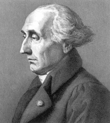
The study of the Brahmagupta–Pell equation reached its pinnacle in the eighteenth century when Lagrange completely described all solutions to this equation using the theory of continued fractions. We briefly explain this theory using an example. Consider the following computations involving \sqrt{7}: \[ \large \sqrt 7 = 2.465…. = 2+ (\sqrt{7}-2) =2+\frac{1}{\frac{1}{\sqrt 7-2}}.\]\[\large \frac{1}{\sqrt 7-2}= 1.548…. = 1+ (\frac{1}{\sqrt 7-2}-1).\]Since \frac{1}{\sqrt 7-2}-1 = (\frac{1 \cdot (\sqrt 7 + 2)}{(\sqrt 7-2) \cdot (\sqrt 7 +2)})-1 = \frac{\sqrt 7-1}{3}, on simplifying, we obtain \frac{1}{\sqrt 7-2}=1+\frac{1}{\frac{3}{\sqrt 7-1}}.
Hence, \[\large
\sqrt 7= 2+\frac{1}{1+\frac{1}{\frac{3}{\sqrt 7-1}}}.
\]
We can repeat this procedure:
\[ \large \frac{3}{\sqrt 7-1}= 1.822…= 1+ (\frac{3}{\sqrt 7-1}-1)=1+ \frac{1}{\frac{2}{\sqrt 7-1}}\]
\[\large
\sqrt 7=2+\cfrac{1}{1+\cfrac{1}{1+\frac{1}{\frac{2}{\sqrt 7-1}}}}
\]
If we continue repeating this procedure, we obtain what is known as the continued fraction of \sqrt{7}:
\[\large
\sqrt 7=2+\cfrac{1}{1+\cfrac{1}{1+\cfrac{1}{ 1+\cfrac{1}{4+\cfrac{1}{1+\cfrac{1}{1+\cfrac{1}{1+\cfrac{1}{4+\cdots}}}}}}}}
\]
As the reader will notice, there is a pattern here: after the initial 2, we get a sequence 1, 1, 1, 4, 1, 1, 1, 4, … in the above continued fraction. As a shorthand, we write \[\large
\sqrt 7= [2; \overline{1, 1, 1, 4}].
\]
The notation above of writing a line above the numbers 1,1,1,4 means that the pattern 1,1,1,4 repeats infinitely many times in the continued fraction representation.
It is a very nice fact that the above method works for any \sqrt{d}, where d is a positive integer: we denote the resulting continued fraction of \sqrt d by [a_0; \overline{a_1, …, a_n}]. We also let \frac{p_m}{q_m}=[a_0; a_1, …, a_m] i.e., \frac{p_m}{q_m} is the truncated continued fraction at the mth stage. For instance, when d=7,
\[\large
\frac{p_3}{q_3}= [2; 1, 1, 1]= 2+\cfrac{1}{1+\cfrac{1}{1+\cfrac{1}{1}}}=\frac{8}{3}.
\]
In the eighteenth century, Lagrange discovered a remarkable connection between continued fractions and the Brahmagupta–Pell equation, which may be stated as follows:
Let d be a positive integer and denote the resulting continued fraction of \sqrt d by [a_0; \overline{a_1, …, a_n}]. For any natural number m, let \frac{p_m}{q_m}=[a_0; a_1, …, a_m]. Then
-
- (p_{n-1}, q_{n-1}) is a solution of x^2-dy^2=1 if n is even.
- (p_{2n-1}, q_{2n-1}) is a solution of x^2-dy^2=1 if n is odd.
- Moreover all positive integer solutions of x^2-dy^2=1 can be obtained from the solution above via the group law.
As an illustrative example, let us take \sqrt{7}. Since \sqrt 7= [2; \overline{1, 1, 1, 4}], we have that n=4. Thus, by Lagrange’s theorem, we conclude that (p_3, q_3) is a fundamental solution. We saw above that \frac{p_3}{q_3}=\frac{8}{3}. Hence, the fundamental solution is (8, 3) and every positive integer solution of x^2-7y^2=1 can be obtained from (8, 3) (by composing it with itself sufficiently many times).
It is interesting to note that the cakravāla method of Bhāskara II also produces the fundamental solution of x^2-dy^2=1 ([9] p.28); it is possible to prove this using ideas from the continued fraction method described above. It is remarkable that the cakravāla method was discovered and used to great effect to solve the Brahamgupta–Pell equation almost 500 years before it was completely solved in Europe.
A binary quadratic form is an expression of the form ax^2+bxy+cy^2, where a, b and c are integers. The discriminant of a binary quadratic form is defined to be D=b^2-4ac.
For a relevant example, we note that the expression x^2-dy^2 is a binary quadratic form with a=1, b=0 and c=-d; therefore the discriminant is 4d.
- We say that a binary quadratic form is primitive if a, b and c are coprime (no integer other than 1 divides a, b and c).
- We say that a binary quadratic form is positive definite if it takes only positive values when x and y are both not zero.
For the rest of this section, we assume that the discriminant of all binary quadratic forms we consider will always be positive. During the study of binary quadratic forms, it was realized that often two quadratic forms are essentially the same. For example, \[\large
x^2+ 2 y^2 \quad \textrm{ and } \quad 2x^2+ y^2
\]just differ up to exchanging the roles of x and y. Similarly,
\[\large
x^2 +2 y^2 \quad \textrm{ and } \quad x^2+2xy+ 3 y^2
\]just differ by the transformation x \mapsto x+y.
We would not like to distinguish between binary quadratic forms appearing in the above examples; in other words, we would like to consider the forms appearing in the above examples as `equivalent’. This intuition is formalized in the following definition:
We say that two binary quadratic forms F(x, y) and F'(x, y) are equivalent if there exists an integer matrix
\[\large \begin{pmatrix}
a & b \\
c & d
\end{pmatrix}\] with determinant equal to 1 such that F(x, y)=F'(ax+by, cx+dy).
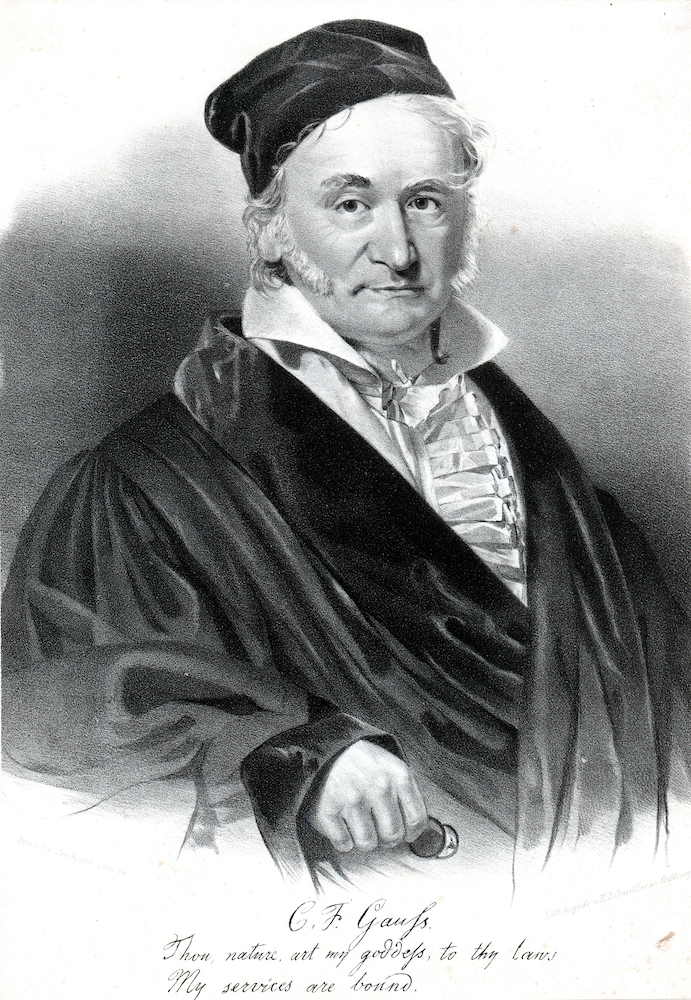
In his masterpiece Disquisitiones Arithmeticae [4] written in 1798, Gauss showed that there are only finitely many equivalence classes of binary quadratic forms with a given discriminant D. He went even further and showed, in a similar spirit to Brahmagupta’s work, that one can “compose’’ two equivalence classes of primitive binary quadratic forms with discriminant D to obtain a third one with the same discriminant. Thus, this composition law equips the set of primitive binary quadratic forms of discriminant D with the structure of an abelian group. This group is called the class group of discriminant D and its size h(D) is called the class number of D.
For example, h(8)=1 as the only primitive binary quadratic form of discriminant 8 up to equivalence is x^2-2y^2.

For instance, the expressions w^2+x^2+ y^2+z^2 and w^2+3x^2+y^2 are quadratic forms.
Moreover, instead of finding integers x and y such that x^2-dy^2 equals 1, we can more generally ask: For any natural number n, when does a quadratic form equal n? There are many results in number theory addressing questions like these; one famous example would be Lagrange’s four-square theorem, which states that for any natural number n, the equation w^2+x^2+y^2+z^2=n always has a solution. In other words, every positive integer can be written as a sum of four squares.
In the setting of the above theorem, we say that the quadratic form w^2+x^2+y^2+z^2 represents all positive integers. Can we find more such examples of quadratic forms which represent all positive integers?
In 1916, Ramanujan [8] gave 54 more examples!
His list starts off with:
\[\large \begin{align*}
w^2+x^2+y^2+2z^2, \quad w^2+x^2+y^2+3z^2 , …,\\w^2+x^2+y^2+7z^2,\quad w^2+x^2+2y^2+3z^2, …
\end{align*}\]
Every example on Ramanujan’s list is correct, except for the quadratic form w^2+ 2x^2+5y^2+5z^2.

\[\large \begin{align*}1, 2, 3, 5, 6, 7, 10, 13, 14, 15, 17, 19, 21, 22, 23, 26,
29,\\ 30,
31, 34, 35, 37, 42, 58, 93, 110, 145, 203, \textrm{ and } 290, \end{align*}\]then it represents all positive integers.
Note that the number 15 appears in the above list and this is consistent with the fact that Ramanujan’s exception does not represent all positive integers.
Summarizing the discussion so far
We hope that this first section has convinced the reader not only of the rich mathematics that the study of the Brahmagupta–Pell equation has given rise to, but also of the remarkable historical continuity of this subject, stretching over a period of approximately 1400 years from Brahmagupta in the seventh century to the present day.
We single out two important facts that we have discussed, since these will play an important role in the remainder of the article:
- The Brahmagupta–Pell equation x^2-dy^2=1 has a fundamental solution which generates all the other solutions.
- For each positive discriminant D, the class number h(D) equals the size of the group of equivalence classes of primitive binary quadratic forms.
Zeta functions
In this section, we introduce zeta functions, which are a class of functions which play a role of paramount importance in modern number theory. While the concepts introduced here might seem slightly technical, we hope the reader will still appreciate their significance and beauty.
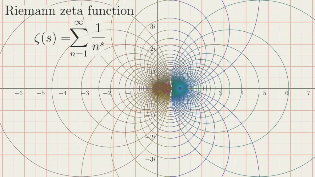
We start with the simplest example of a zeta function: the Riemann zeta function. For a complex number s, the Riemann zeta function is the infinite series
\[\large
\zeta(s)= \sum_{n=1}^{\infty} \frac{1}{n^s}= \frac{1}{1^s}+\frac{1}{2^s}+\frac{1}{3^s}+ \cdots
\]This series converges3 when the real part of s (denoted \textrm{Re}(s)) is larger than one, and defines a holomorphic function4 on this region.
Even though this function is named after Riemann, it was studied extensively by Euler. For example, Euler evaluated this function at even numbers and obtained beautiful formulas such as
\[\large \begin{align*}
\zeta(2)=\frac{1}{1^2}+\frac{1}{2^2}+\frac{1}{3^2}+\frac{1}{4^2}+ \cdots = \frac{\pi^2}{6},\quad
\zeta(4)=\frac{1}{1^4}+\frac{1}{2^4}+\frac{1}{3^4}+\frac{1}{4^4}+ \cdots = \frac{\pi^4}{90},\\
\mathrm{ and}\quad
\zeta(6)=\frac{1}{1^6}+\frac{1}{2^6}+\frac{1}{3^6}+\frac{1}{4^6}+ \cdots = \frac{\pi^6}{945}.
\end{align*}\]In general, Euler gave an explicit formula for the value of \zeta(s) at an even positive integer: he showed that
\[\large
\zeta(2k)=\frac{1}{1^{2k}}+\frac{1}{2^{2k}}+\frac{1}{3^{2k} }+ \frac{1}{4^{2k}}+ \cdots = \pi^{2k} \cdot x,
\]where x is a rational number which can be described explicitly (in terms of the celebrated Bernoulli numbers).5
Euler also discovered the following remarkable fact: even though \zeta(s) is defined as an infinite sum over natural numbers, it can also be written as an infinite product over prime numbers. More precisely, he showed that if \textrm{Re}(s)>1, then
\[\large \begin{align*}
\zeta(s) &=
\prod_{p} \left (1-\frac{1}{p^s} \right) ^{-1}\\
&= \left (1-\frac{1}{2^s} \right) ^{-1} \cdot \left (1-\frac{1}{3^s} \right) ^{-1} \cdot \left (1-\frac{1}{5^s} \right) ^{-1} \cdots
\end{align*}\]
Let us briefly explain the idea behind this fact by successively simplifying the expression. We first note that when we multiply \zeta(s) by \left (1-\frac{1}{2^s} \right), all the terms corresponding to the even numbers disappear:
\[\large \begin{align*}
&\left (1-\frac{1}{2^s} \right) \zeta(s)\\
& = \left (\frac{1}{1^s}+\frac{1}{2^s}+\frac{1}{3^s} +\cdots \right) – \left(\frac{1}{2^s}+\frac{1}{4^s}+\frac{1}{6^s} +\cdots \right)\\
& = \frac{1}{1^s}+ \frac{1}{3^s}+\frac{1}{5^s}+\frac{1}{7^s} + \cdots
\end{align*}\]If we now multiply the above expression with \left (1-\frac{1}{3^s} \right), we see that all the terms corresponding to multiples of 3 disappear. Indeed:
\[\large \begin{align*}
&\left (1-\frac{1}{3^s} \right) \left (1-\frac{1}{2^s} \right) \zeta(s)\\
& = \left (\frac{1}{1^s}+\frac{1}{3^s}+\frac{1}{5^s} +\cdots \right) – \left(\frac{1}{3^s}+\frac{1}{9^s}+\frac{1}{15^s} +\cdots \right)\\
&= \frac{1}{1^s}+ \frac{1}{5^s}+\frac{1}{7^s} + \frac{1}{11^s} \cdots.
\end{align*}\]Euler observed that if we continue this procedure for all primes p, the only term that remains is the number 1, that is,
\[\large
\prod_p \left (1- \frac{1}{p^s} \right) \zeta(s) =1
\]and so \zeta(s) = \prod_{p} \left (1-\frac{1}{p^s} \right) ^{-1} as claimed. This expression takes the shape
\[\large \begin{align*}
\boxed{\textrm{A sum over natural numbers} }
= \boxed{\textrm{A product over prime numbers}}
\end{align*}\]and reflects the harmony that exists in the world of numbers. In honour of Euler, any expression in number theory that assumes such a form is known as an Euler product.
As mentioned above, \zeta(s) only converges when \textrm{Re}(s)>1; however, Euler also developed a method to sum the divergent series obtained when we substitute negative values in the definition of \zeta(s). For example, Euler substituted s=-1, s=-2 and s=-3 in the definition of \zeta(s) and claimed that
\[\large \begin{align*}
1+2+3+4+ \cdots =-\frac{1}{12}, \quad 1^2+2^2+3^2+4^2+ \cdots =0 \quad \textrm{and} \quad 1^3+2^3+3^3+4^3+ \cdots=\frac{1}{120}
\end{align*}\]Remarkably, these exact same formulas were written down by Ramanujan in his famous letter ([1] p.21) to Hardy in 1913. Although these formulas are not literally correct, there is a sense in which they are true. To explain this, we mention that Riemann in 1859 found a new holomorphic function which is defined on all complex numbers.6 This function agrees with \zeta(s) when \textrm{Re}(s)>1. It is standard to call this new function \zeta(s) as well; in other words, Riemann found a way to extend the definition of the original function (which was only defined for \textrm{Re}(s)>1) to all complex numbers. This process is termed “analytic continuation” in modern terminology and via this process, it turns out that indeed
\[\large
\zeta(-1) = -\frac{1}{12}, \hspace{5mm} \zeta(-2)=0 \hspace{5mm} \textrm{and} \hspace{5mm} \zeta(-3)=\frac{1}{120}.
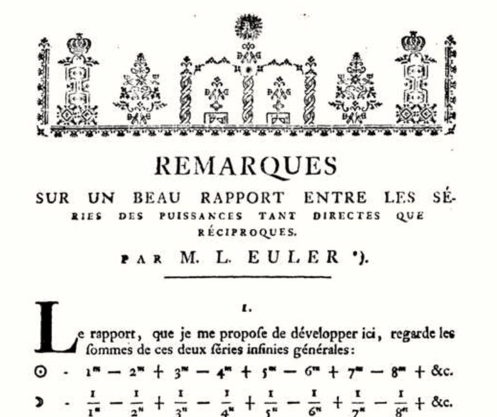
\]Euler also noticed a remarkable duality between the values of the zeta function at negative integers and positive integers. In his 1749 paper Remarques sur un beau rapport entre les séries des puissances tant directes que réciproques [3] (translated as `Remarks on a beautiful relationship between the power series, direct as well as reciprocal’), he poetically expressed this duality to be similar to the duality between the sun and the moon: for any positive integer m, he defined the “sun series”
\[\large
\odot: 1^m-2^m+3^m-4^m+5^m- \cdots
\]and for any positive integer n, he defined the “moon series”
\[\large
☽ : \frac{1}{1^n}-\frac{1}{2^n}+\frac{1}{3^n}-\frac{1}{4^n}+\frac{1}{5^n}- \cdots
\]Note that the series \odot is closely related (but not quite equal, due to the presence of alternating negative signs) to the values of \zeta(s) at negative integers and similarly, ☽ is closely related to the values of \zeta(s) at positive integers.
For n=1+m, Euler proved the relation
\[\large
\frac{\odot}☽= – \frac{1 \cdot 2 \cdot 3 \cdots (n-1)}{ (2^{n-1}-1) \pi^n } (2^n-1) \cos \left (\frac{n \pi}{2} \right).
\]
In other words, the values of \zeta(s) at negative integers and the values of \zeta(s) at positive integers are related. Riemann showed that something much more is true: for any complex number s, the value of \zeta(s) and \zeta(1-s) are related in a precise way:
\[\large
\pi^{-(1-s)/2} \Gamma \left( \frac{1-s}{2} \right) \zeta(1-s)= \pi^{-s/2} \Gamma \left( \frac{s}{2} \right) \zeta(s),
\]
This formula, giving us a symmetry \zeta(s) \longleftrightarrow \zeta(1-s), is known as the functional equation for the Riemann zeta function.
Let us briefly summarize our discussion so far. We have defined the Riemann zeta function \zeta(s)=\sum_{n=1}^{\infty} \frac{1}{n^s} and seen that it satisfies three key properties:
- it has an Euler product,
- its definition can be extended to the entire complex plane and
- it has a functional equation relating \zeta(s) to \zeta(1-s).
Let N be a natural number. A Dirichlet character mod N is a function
\[\large
\chi: \mathbb N \rightarrow \mathbb C
\]with the following three properties:
- \chi is invariant under addition by N, i.e., \chi(n +N)=\chi(n),
- \chi is multiplicative, i.e., \chi(m n)= \chi(m) \cdot \chi(n), and
- \chi(n)=0 whenever n and N are not coprime (i.e., n and N share a common factor greater than 1).
Let us demystify the above definition by means of an example. Consider the function
\[\large
\chi_4: \mathbb N \rightarrow \mathbb C
\]given by
\[ \large \chi_4(n)= \begin{cases}
0 & \textrm{ if } n \textrm{ is even} \\
1 & \textrm{ if } n=4k+1 \textrm{ for some } k \\
-1 & \textrm{ if } n=4k+3 \textrm{ for some } k \\
\end{cases}
\]
We invite the reader to check that \chi_4 indeed satisfies the definition of a Dirichlet character mod 4.
Given a Dirichlet character \chi, the zeta function associated to \chi is defined as
\[\large
L(\chi, s) = \sum_{n=1}^{\infty} \frac{\chi(n) }{n^s}
\]and is called the Dirichlet L-function associated to \chi.
In number theory, the terms zeta functions and L-functions are used interchangeably. In this case, it is standard terminology to call L(\chi, s) a Dirichlet L-function rather than a Dirichlet zeta function and to denote the function by the letter “L” rather than the letter “\zeta“.7 The Dirichlet L-function also satisfies the three key properties of zeta functions that we discussed earlier in this section:
- it has an Euler product, which takes the shape
- its definition can be extended to all complex numbers, and
- it has a functional equation giving us a relation between values at s and 1-s.
\[\large
L(\chi, s) = \prod_p (1 – \chi(p) p^{-s})^{-1},
\]
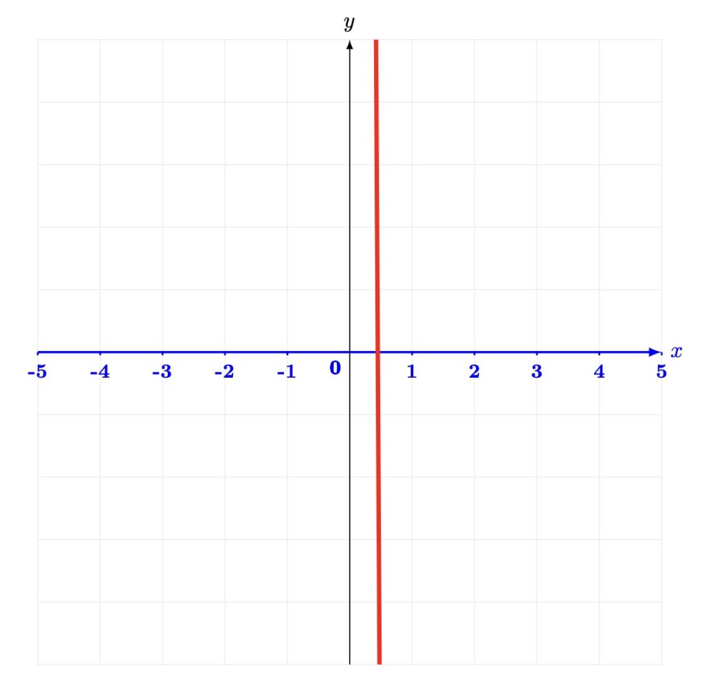
However, instead of studying the values of zeta functions on the vertical line \textrm{Re}(s)=\frac{1}{2}, which is the focus of the Riemann hypothesis, we can also study the values of zeta functions on the horizontal line \textrm{Im}(s)=0 i.e., the x-axis. This line is special since it contains all the integers; evaluating zeta functions at integers leads us to another important theme in modern number theory, and the main subject of this article: special values of zeta functions. In the context of this article, we will indicate the surprising connections of this theme with the Brahmagupta–Pell equation.
\[\large \boxed{\textbf{Special values of zeta functions is the study of the values of zeta functions at integers.}}\]For instance, Euler’s formula
\[\large
\zeta(2)=\frac{1}{1^2}+\frac{1}{2^2}+\frac{1}{3^2}+\frac{1}{4^2}+ \cdots = \frac{\pi^2}{6}
\]is an example of a special value of a zeta function. These kinds of formulas often have very deep meanings: for example, this formula can be used to show two amazing facts:
- The probability that two random positive integers are coprime (share no common factor) is \frac{6}{\pi^2}.
- The probability that a random positive integer is square-free (not divisible by any square number other than one) is also \frac{6}{\pi^2}.
Since \frac{6}{\pi^2} \approx 0.61, we can conclude for instance that there is a 61% chance that a positive integer is square-free. The values of the Riemann zeta function at other integers also carry a tremendous amount of interesting information and have led to many exciting developments in number theory.
We will now focus on the value of Dirichlet L-functions at s=1 and explain a result that is often regarded as one of the earliest theorems in the area of special values of zeta functions: the analytic class number formula.
Subsequently, we will tie our discussion back to the material discussed in the first section and see, quite unexpectedly, that the values of Dirichlet L-functions at s=1 are closely related to the Brahmagupta–Pell equation.
The analytic class number formula
We begin by choosing a square-free positive integer d such that either d-2 or d-3 is divisible by 4 (such as 6 or 7). Consider the Brahmagupta–Pell equation
\[\large
x^2-dy^2=1.
\]Up to now, we have been interested in finding integer solutions to this equation. But, as is often the case in number theory, we can also look for solutions `mod p‘ for a prime number p; in other words, we can look for solutions to this equation in the group \mathbb Z/p \mathbb Z. This refers to solutions (x,y) such that 0 \leq x,y \leq p-1 and x^2 - dy^2 - 1 is divisible by p.
For example, when p=3 and d=7, the equation x^2-dy^2=1 has two solutions mod p: (1, 0) and (2, 0). Indeed, we only need to try x \in \{0,1, 2\} and y \in \{0, 1, 2\} and check when x^2-dy^2-1 is divisible by p. A quick check gives us the two solutions above.
When \frac{d}{p} is not an integer, it is a fact that x^2-dy^2=1 always has either p-1 or p+1 solutions mod p.
Define a function \chi_d on all prime numbers p via
\[ \large \chi_d (p)=\begin{cases}
1 & \textrm{ if } x^2- dy^2=1 \textrm{ has } p-1 \textrm{ solutions mod }p \\
-1 & \textrm{ if } x^2- dy^2=1 \textrm{ has } p+1 \textrm{ solutions mod }p \\
0 & \textrm{ if } {d \textrm{ is a multiple of }p} \\
\end{cases}
\]and extend it to all of \mathbb N by multiplicativity. Using the law of quadratic reciprocity, a beautiful theorem in number theory, one can show that \chi_d is a Dirichlet character mod 4d. We may thus consider the Dirichlet L-function L(\chi_d, s).
In a celebrated result from 1839, known as the analytic class number formula, Dirichlet showed that
\[\large
L(\chi_d, 1)= \frac{ h(4d) \cdot \log (a+b \sqrt d ) }{2 \sqrt d},
\]where (a, b) is a fundamental solution of x^2-dy^2=1 and h(4d) is the class number of discriminant 4d.
Thus, the Dirichlet L-function L(\chi_d, s) captures information about the fundamental solution of x^2-dy^2=1 and the class number of discriminant 4d, both of which, as we saw in the first section of the article, are of central importance in number theory. This is just one example of a theme that shows up time and time again in modern number theory: zeta functions always seem to appear in mysterious ways whenever we study important concepts and problems in number theory. We give a brief indication of this in the next section.
Before doing so, we briefly explain two features of the analytic class number formula which showcase, despite only being the first result in the area of special values of zeta functions, its incredible depth and beauty. Firstly, the analytic class number formula has the shape
\[\large
\boxed{\textrm{Analytic} } = \boxed{\textrm{Algebraic}}
\]The left-hand side is completely analytic in nature: it is the value of a holomorphic function at a point, such as a special value of a zeta function On the other hand, the right side involves quantities such as the class number and fundamental solution of an equation such as the Brahmagupta–Pell equation; it is thus very algebraic in nature.
Secondly, this formula also has the shape
\[\large
\boxed{\textrm{Local}} = \boxed{\textrm{Global}}
\]The Dirichlet L-function on the left-hand side was defined via \chi_d which was in turn defined by counting how many solutions the Brahmagupta–Pell equation has mod p for every prime p; it is thus something defined locally i.e., prime by prime. But, quite mysteriously, via the analytic class number formula, this L-function also embodies global (i.e., independent of any prime) information: its value at 1 yields the fundamental solution of the Brahmagupta–Pell equation and the class number of quadratic forms, which are both global quantities.
While the proof of the above formula is outside the scope of this article, we remark that it involves a marvellous synthesis of algebra and analysis. We particularly recommend [7] as an excellent source for further information on the analytic class number formula and for other developments discussed in the article.
The Birch and Swinnerton-Dyer conjecture and beyond

It is also possible to attach a zeta function L(E, s) to the elliptic curve (in this case also, it is more common to denote the function by L rather than \zeta and call the function an L-function). As with the zeta functions we have seen before, L(E, s) is a holomorphic function on the entire complex plane and hence admits a Taylor-series expansion at s=1:
\[\large L(E, s)= c_0+ c_1(s-1)+c_2(s-1)^2+ \cdots \]The least i such that c_i \neq 0 is called the order of vanishing of the L-function at s=1 and is denoted by \textrm{ord}_{s=1} L(E, s).
The Birch and Swinnerton-Dyer conjecture, one of the seven Clay Millennium Prize problems,10 predicts that for an elliptic curve E, \textrm{ord}_{s=1} L(E, s)= r_E. In other words, the conjecture predicts that the order of vanishing of the L-function at s=1 equals the rank of the elliptic curve.11
Thus, this conjecture is another illustration of the intertwinement between algebraic and analytic quantities in number theory: the order of vanishing is defined via analysis, while the rank is defined completely via algebra. We wish to emphasize that this interaction between algebraic and analytic viewpoints is a fundamental theme of modern number theory, and as we saw before, the seeds of this theme can be traced back to the study of the Brahmagupta–Pell equation.
Note that the Birch and Swinnerton-Dyer conjecture predicts that L(E, 1)=0 if and only if r_E \geq 1; so L(E, 1)=0 if and only if E has infinitely many rational points. Just like the analytic class number formula, knowing the value of L(E, s) at s=1 gives us information about integer or rational solutions to the equation we started off with!
To make the analogy with the class number more precise, we remark that there is also a refined version of the Birch and Swinnerton-Dyer conjecture which predicts that the leading term in the Taylor series expansion of L(E, s) at s=1 (i.e., the value of c_i for the least i such that c_i \neq 0) is given by
\[\large
\frac{\#\mathrm{Sha}(E) \cdot \Omega_E \cdot R_E \cdot \prod_{p|N}c_p}{(\#E_{\mathrm{Tor}})^2}.
\]While we do not explain the meaning of the terms appearing here, we remark that the quantity \# \mathrm{Sha}(E) is an analogue of the class number and the quantity R_E is an analogue of the logarithm of the fundamental solution of the Brahmagupta–Pell equation. Thus, the Birch and Swinnerton-Dyer conjecture can be thought of as an analogue of the class number formula for elliptic curves. While partial progress has been made on this conjecture, it remains wide open today.
Quite remarkably, there is a wide-reaching conjecture known as the Bloch–Kato conjecture that subsumes both the analytic class number formula and the Birch and Swinnerton-Dyer conjecture as special cases. Instead of considering just the Brahmagupta–Pell equation (which is a quadratic equation) or elliptic curves (which are cubic equations), the conjecture considers general algebraic varieties, which are degree n equations for a natural number n. Just like the analytic class number formula and the Birch and Swinnerton-Dyer conjecture, the Bloch–Kato conjecture makes a precise prediction about how the zeta function attached to an algebraic variety captures information about certain fundamental quantities related to the algebraic variety. The mathematician Kazuya Kato, whose name appears in the above conjecture, wrote a book (along with Nobushige Kurokawa and Takeshi Saito) entitled Number Theory 1: Fermat’s Dream [6]. This book gives an excellent introduction to many important topics in modern number theory. As one might expect, there is a chapter on zeta functions. However, the chapter is named “\zeta” rather than “\zeta functions”; the authors explain why this is the case ([6] p.84):
This quote embodies the main message of this article very well: even though \zeta functions are just functions, they are profound and mysterious mathematical objects that hold the key to unlocking many secrets of number theory. We are still very far away from understanding the true meaning of zeta functions; nevertheless, we are making rapid progress and it is likely the future holds many exciting discoveries as we continue in our quest to understand zeta functions. It is remarkable that an equation studied by Brahmagupta nearly 1400 years ago provides us with an inroad into this quest.
Acknowledgements: I am very grateful to C.S. Aravinda and the editorial team at Bhāvanā for very helpful feedback on a previous draft of this article. \blacksquare
References
- [1] B. Berndt and R. Rankin, Ramanujan: Letters and Commentary, a co-publication of the American Mathematical Society and London Mathematical Society, 1995.
- [2] M. Bhargava and J. Hanke, Universal quadratic forms and the 290-theorem, 2005, preprint.
- [3] L. Euler, Remarques sur un beau rapport entre les séries des puissances tant directes que réciproques, published in 1768.
- [4] C.F. Gauss, Disquisitiones Arithmeticae, 1801 (English translation by Arthur A. Clarke, Yale University Press, 1965).
- [5] J. Lagrange, Recherches d’arithmetique, Nouveaux Mémoires de l’académie des sciences de Berlin, Volume 5, 1775, 265–312.
- [6] K. Kato, N. Kurokawa, and T. Saito, Number Theory 1: Fermat’s Dream, American Mathematical Society, Providence, Rhode Island, 2011. Originally published in Japanese by Iwanami Shoten Publishers, Tokyo, 1996. Translated from Japanese by Masato Kuwata.
- [7] J. Stopple, A Primer of Analytic Number Theory: From Pythagoras to Riemann, Cambridge University Press, 2003.
- [8] S. Ramanujan, On the expression of a number in the form ax^2+by^2+cz^2+du^2, Proc. Camb. Phil. Soc. 19 (1916), pp. 11–21.
- [9] V.S. Varadarajan, Algebra in ancient and modern times, a co-publication of the American Mathematical Society and the Hindustan Book Agency, 1998.
Footnotes
- Editor’s note: While this article could be slightly more technical than the usual Bhāvanā articles, it still has a strong flavour of outreach, which remains our main motto. We believe that more than half of the article should still be accessible to our general readership, possibly with a bit of extra effort or help, and is a great read nevertheless. ↩
- A group is a mathematical structure consisting of a set in which any two elements can be composed via an operation, such as addition or multiplication or some other mathematical operation, to produce another element of the same set. In this case, we see how two solutions of the Brahmagupta–Pell equation are composed to produce a third solution. This composition rule thus induces a mathematical operation on the set of all solutions to the Brahmagupta–Pell equation, to render it with the structure of a group. ↩
- that is, sums up to a finite number. ↩
- An analogue of a differentiable function for functions defined on complex numbers. ↩
- Bernoulli numbers are special numbers that appear in the power series of some trigonometric functions. Their connection with special values of zeta functions is a fascinating area of study. ↩
- Strictly speaking, \zeta(s) is defined on all complex numbers except for s=1. ↩
- We note here that the Riemann zeta function is a special example of a Dirichlet L-function. If we define \chi to be the trivial character that takes the value 1 whenever n is coprime to N, then L(\chi,s) is the product of \zeta(s) and a quantity that captures the prime divisors of N. ↩
- \zeta(s) also has zeros at all negative even integers. These are often called “trivial zeros” of \zeta(s) and are not the focus of the Riemann hypothesis. Similarly, L(\chi, s) also has trivial zeros at either all the negative even integers or at all the negative odd integers. ↩
- To be slightly more precise, the group of rational points E(\mathbb Q) is a finitely generated abelian group and so, by the structure theory of finitely generated abelian groups, E(\mathbb Q)=\mathbb Z^r \oplus T, for some r \in \mathbb N and some finite group T. We define r_E:=r. ↩
- A list of extremely challenging mathematical problems collected by the Clay Mathematics Institute; for the solution of each of these problems, the Clay Institute has announced a reward of 1 million US dollars. ↩
- We refer the interested reader to the recent interview we featured with Don Zagier, in which he discusses, among several important themes in modern number theory, the Birch and Swinnerton-Dyer conjecture. The interview can be accessed at https://bhavana.org.in/speaking-the-language-of-mathematics/. ↩